Tutorial 1: Vector Analysis
Vector data can also be analyzed to reveal how different features interact with each other in space. There are many different analysis-related functions in GIS, so we won’t go through them all. Rather, we’ll pose a question and try to solve it using the tools that QGIS provides.
The goal for this lesson: To ask a question and solve it using analysis tools.
1.  The GIS Process
Before we start, it would be useful to give a brief overview of a process that can be used to solve any GIS problem. The way to go about it is:
- State the Problem
- Get the Data
- Analyze the Problem
- Present the Results
2. The Problem
Let’s start off the process by deciding on a problem to solve. For example, you are an estate agent and you are looking for a residential property in Swellendam for clients who have the following criteria:
- It needs to be in Swellendam
- It must be within reasonable driving distance of a school (say 1km)
- It must be more than 100m squared in size
- Closer than 50m to a main road
- Closer than 500m to a restaurant
3. The Data
To answer these questions, we’re going to need the following data:
- The residential properties (buildings) in the area
- The roads in and around the town
- The location of schools and restaurants
- The size of buildings
All of this data is available through OSM and you should find that the dataset you have been using in lab 2 can also be used here.
If you want to download data from another area you can find more information in QGIS official manual.
Note
Although OSM downloads have consistent data fields, the coverage and detail does vary. If you find that your chosen region does not contain information on restaurants, for example, you may need to chose a different region.
4. Follow Along: Start a Project and get the Data
We first need to load the data to work with. This time we will load data from a GeoPackage file, which is a container that allows you to store GIS data (layers) in a single file. Unlike the ESRI Shapefile format (e.g. all the .shp datasets you used earlier), a single GeoPackage file can contain various data (both vector and raster data) in different coordinate reference systems, as well as tables without spatial information; all these features allow you to share data easily and avoid file duplication.
Download this GeoPackage file.
Create a new map.
Click on the
 Open Data Source Manager button.
On the left click on the GeoPackage tab.
-
Click on the New button and browse to the
lab5tutorial1.gpkgfile you downloaded before. Select the file and press
Open. The file path is now added to the Geopackage connections list, and appears in the drop-down menu.You are now ready to add any layer from this GeoPackage to QGIS.
-
Click on the Connect button. In the central part of the window you should now see the list of all the layers contained in the GeoPackage file.
Select any of the layers and click on the Add button.
You will see that the layer has been added to the Layers panel with features displayed on the map canvas.
Using the same approach you can add all other layers from the file (you can also add them all simultaneously by selecting them with Shift key).
If you want you can add a background map. Open the Browser and load the OSM background map from the XYZ Tiles menu.
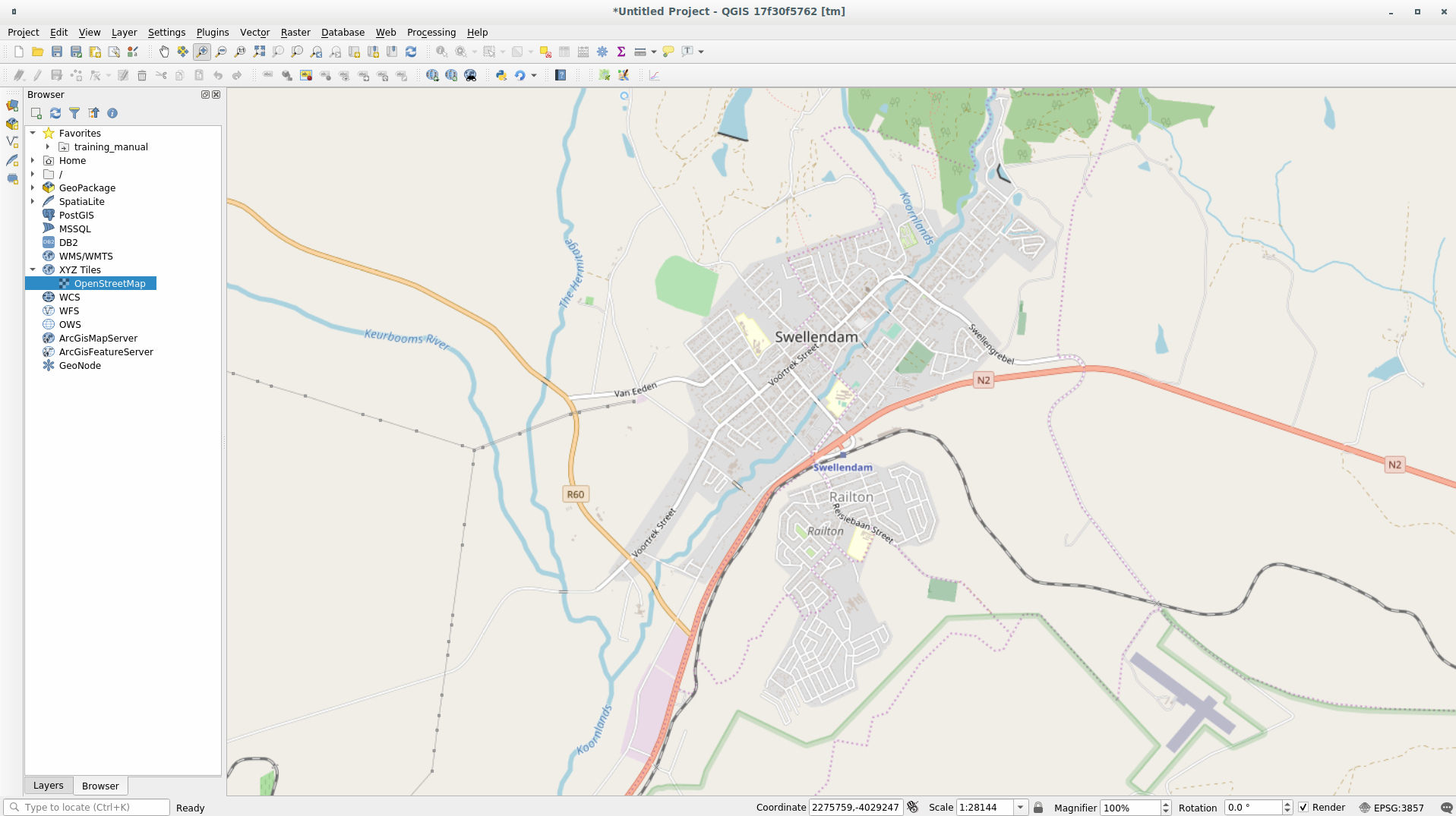
Zoom to the layer extent to see Swellendam, South Africa
Before proceeding we should filter the roads layer in order to have only some specific road types to work with.
Some of the roads in OSM dataset are listed as unclassified, tracks,
path and footway. We want to exclude these from our dataset and focus on
the other road types, more suitable for this exercise.
Moreover, OSM data might not be updated everywhere and we will also exclude
NULL values.
Right click on the roads layer and choose Filter….
In the dialog that pops up we can filter these features with the following expression:
"highway" NOT IN ('footway','path','unclassified','track') OR "highway" != NULL
The concatenation of the two operators
NOTandINmeans to exclude all the unwanted features that have these attributes in thehighwayfield.!= NULLcombined with theORoperator is excluding roads with no values in thehighwayfield.You will note the
 icon next to the roads layer
that helps you remember that this layer has a filter activated and not all the
features are available in the project.
icon next to the roads layer
that helps you remember that this layer has a filter activated and not all the
features are available in the project.

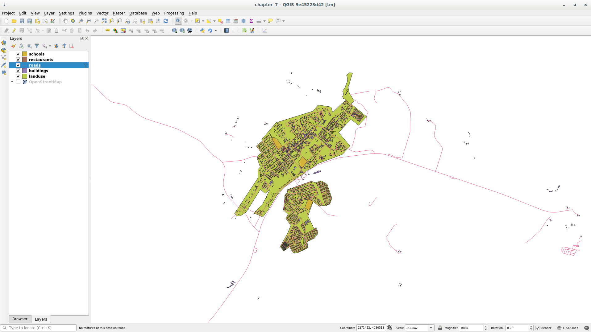
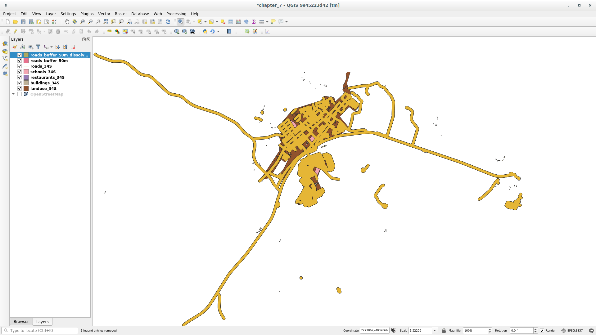
The map with all the data should look like the following one:
5. Try Yourself Convert Layers’ CRS
Because we are going to be measuring distances within our layers, we need to change the layers’ CRS. To do this, we need to select each layer in turn, save the layer to a new one with our new projection, then import that new layer into our map.
You have many different options, e.g. you can export each layer as a new
Shapefile, you can append the layers to an existing GeoPackage file or you can
create another GeoPackage file and fill it with the new reprojected layers. We
will show the last option so the training_data.gpkg will remain clean.
But feel free to choose the best workflow for yourself.
Note
In this example, we are using the WGS 84 / UTM zone 34S CRS, but you may use a UTM CRS which is more appropriate for your region.
Right click the roads layer in the Layers panel;
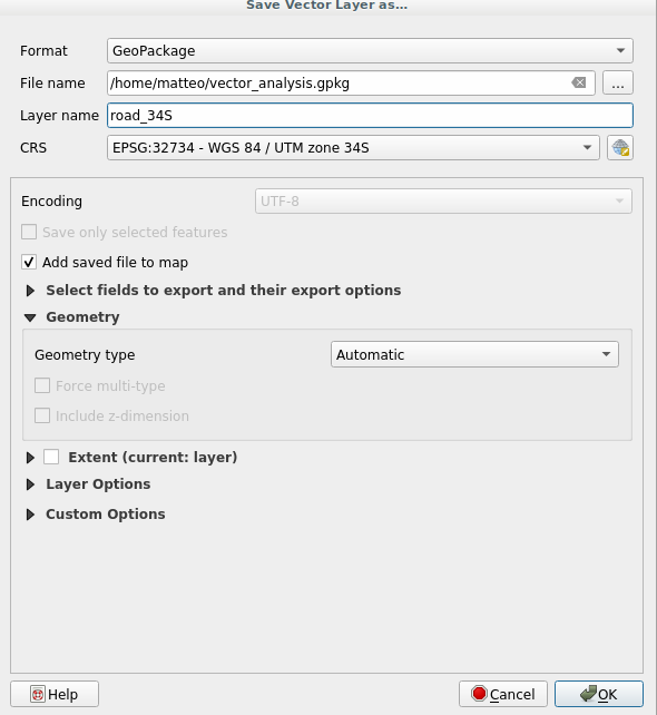
Click Export –> Save Features As…;
In the Save Vector Layer As dialog choose GeoPackage as Format;
Click on … of File name parameter and name the new GeoPackage as vector_analysis;
Change the Layer name as roads_34S;
Change the CRS parameter to WGS 84 / UTM zone 34S;
Finally click on OK:
This will create the new GeoPackage database and fill it with the roads_34S layer.
Repeat this process for each layer, creating a new layer in the
vector_analysis.gpkgGeoPackage file with_34Sappended to the original name and removing each of the old layers from the project.Note
When you choose to save a layer to an existing GeoPackage, QGIS will append that layer in the GeoPackage.
Once you have completed the process for each layer, right click on any layer and click Zoom to layer extent to focus the map to the area of interest.
Now that we have converted OSM’s data to a UTM projection, we can begin our calculations.
6. Follow Along: Analyzing the Problem: Distances From Schools and Roads
QGIS allows you to calculate distances from any vector object.
Make sure that only the roads_34S and buildings_34S layers are visible, to simplify the map while you’re working
Click on the to open the analytical core of QGIS. Basically: all algorithms (for vector and raster) analysis are available within this toolbox.
We start by calculating the area around the roads_34S by using the Buffer algorithm. You can find it expanding the group.
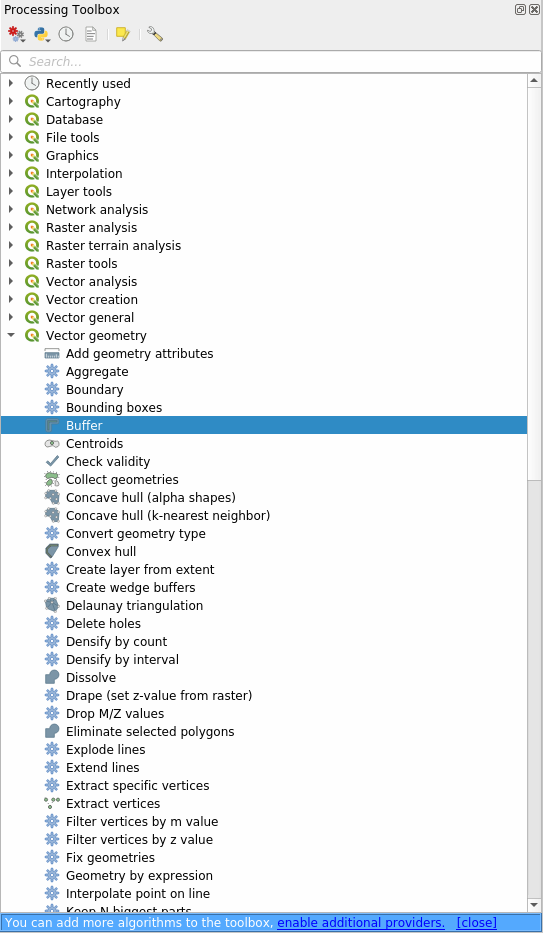
Or you can type
bufferin the search menu in the upper part of the toolbox: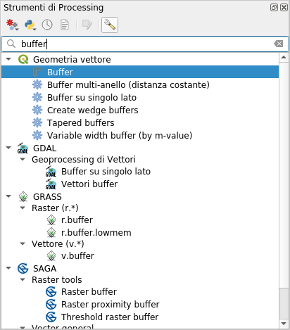
Double click on it to open the algorithm dialog
Set it up like this
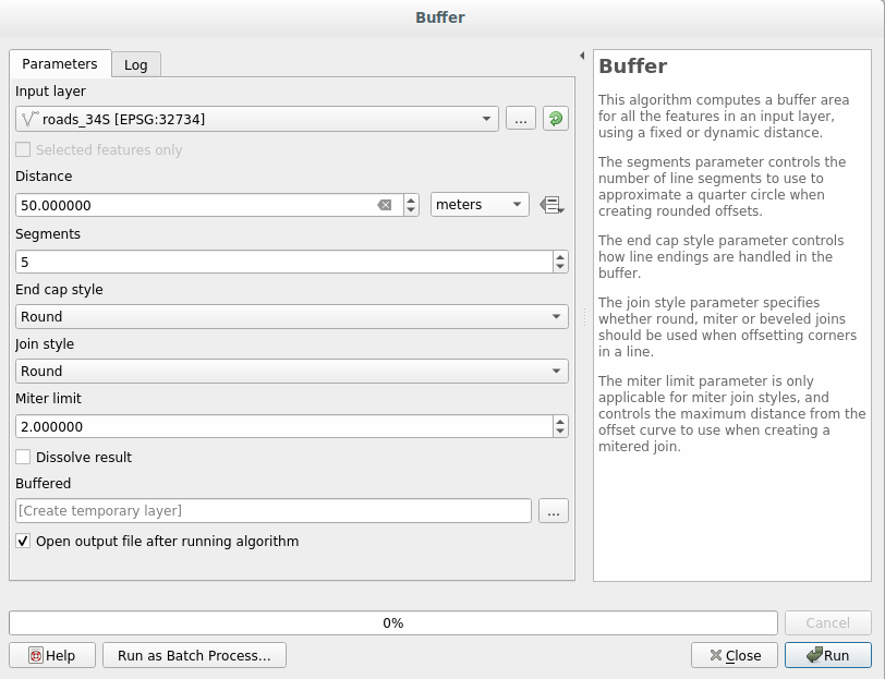
The default Distance is in meters because our input dataset is in a Projected Coordinate System that uses meter as its basic measurement unit. You can use the combo box to choose other projected units like kilometers, yards, etc.
Note
If you are trying to make a buffer on a layer with a Geographical Coordinate System, Processing will warn you and suggest to reproject the layer to a metric Coordinate System.
By default Processing creates temporary layers and adds them to the Layers panel. You can also append the result to the GeoPackage database by:
- clicking on the … button and choose Save to GeoPackage…
- naming the new layer roads_buffer_50m
- and saving it in the
vector_analysis.gpkgfile

Click on Run and then close the Buffer dialog.
Now your map will look something like this:
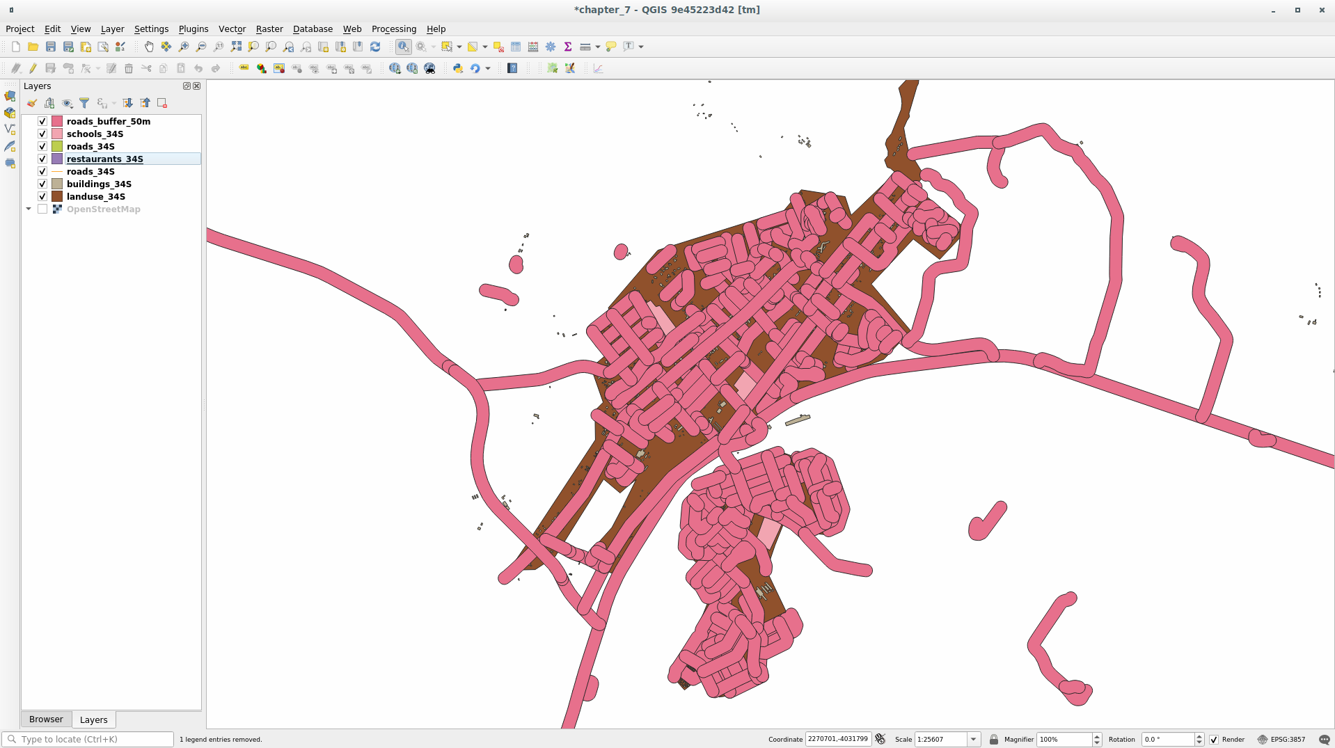
If your new layer is at the top of the Layers list, it will probably obscure much of your map, but this gives you all the areas in your region which are within 50m of a road.
However, you’ll notice that there are distinct areas within your buffer, which correspond to all the individual roads. To get rid of this problem:
Uncheck the roads_buffer_50m layer and re-create the buffer using the settings shown here:
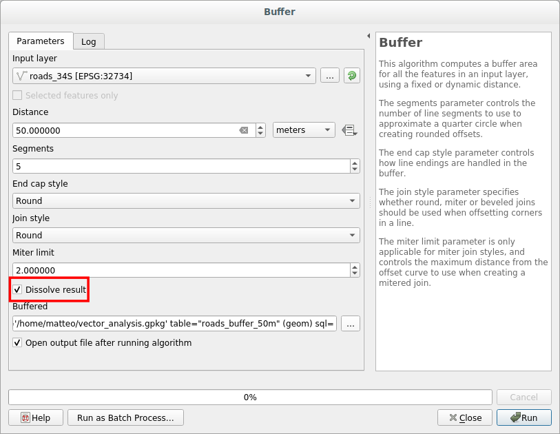
Note that we’re now checking the Dissolve result box
Save the output as roads_buffer_50m_dissolved
Click Run and close the Buffer dialog again
Once you’ve added the layer to the Layers panel, it will look like this:
Now there are no unnecessary subdivisions.
Note
The Short Help on the right side of the dialog explains how the algorithm works. If you need more information, just click on the Help button in the bottom part to open a more detailed guide of the algorithm.
7. Try Yourself Distance from schools
Use the same approach as above and create a buffer for your schools.
It needs to be 1 km in radius. Save the new layer in the
vector_analysis.gpkg file as schools_buffer_1km_dissolved.
8. Follow Along: Overlapping Areas
Now we have areas where the road is 50 meters away and there’s a school within 1 km (direct line, not by road). But obviously, we only want the areas where both of these criteria are satisfied. To do that, we’ll need to use the Intersect tool. You can find it in group within .
Set it up like this:
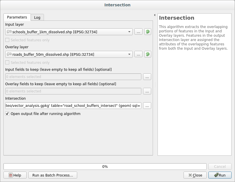
- The input layers are the two buffers
- The saving location is, once again, the
vector_analysis.gpkgGeoPackage - And the output layer name is road_school_buffers_intersect
Click Run.
In the image below, the blue areas show us where both distance criteria are satisfied at once!
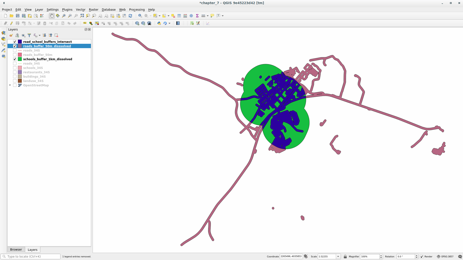
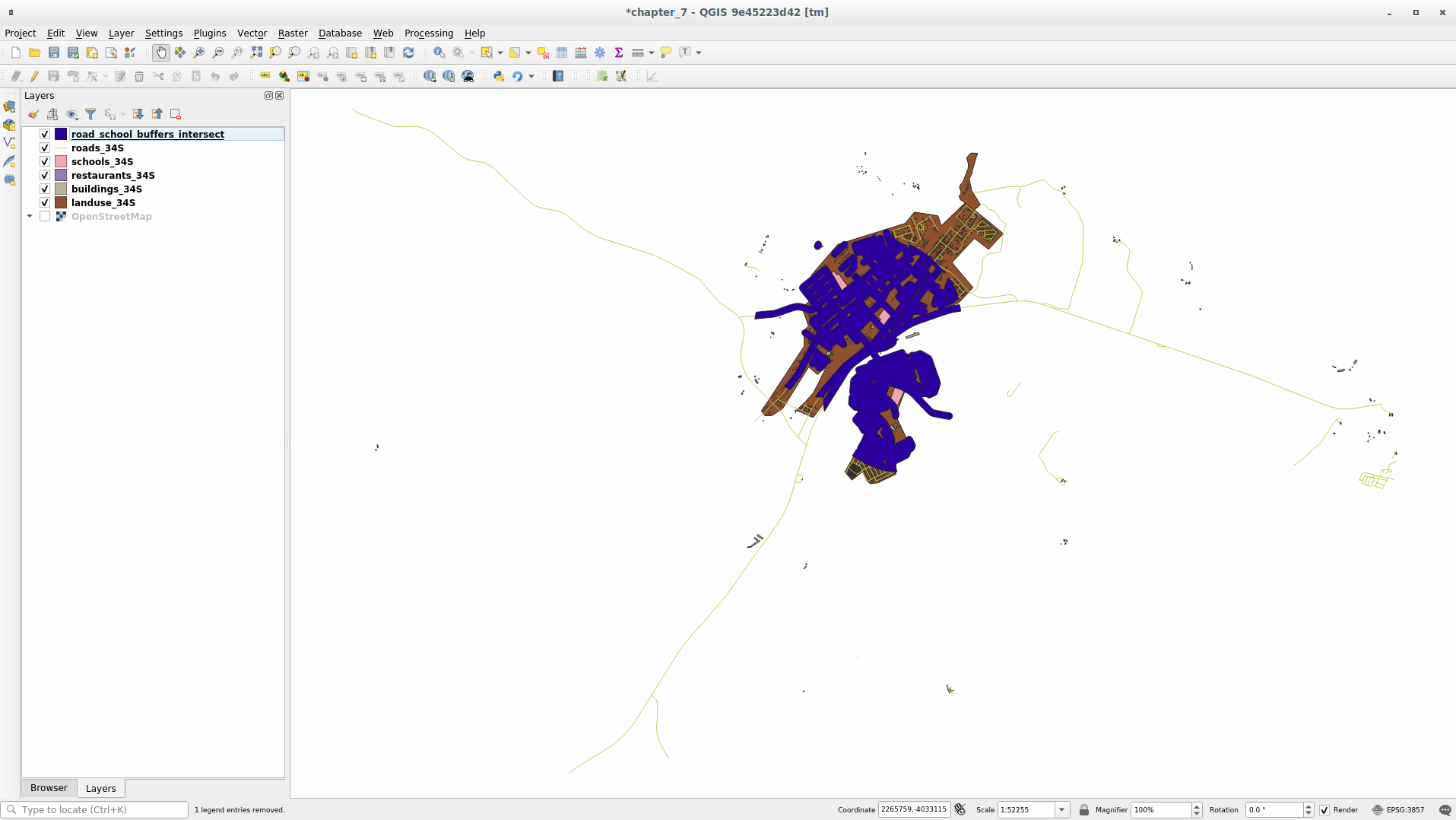
You may remove the two buffer layers and only keep the one that shows where they overlap, since that’s what we really wanted to know in the first place:
9. Follow Along: Extract the Buildings
Now you’ve got the area that the buildings must overlap. Next, you want to extract the buildings in that area.
Look for the menu entry within
Set up the algorithm dialog like in the following picture
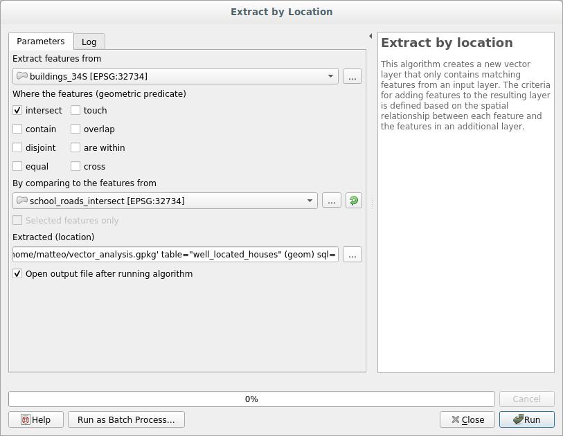
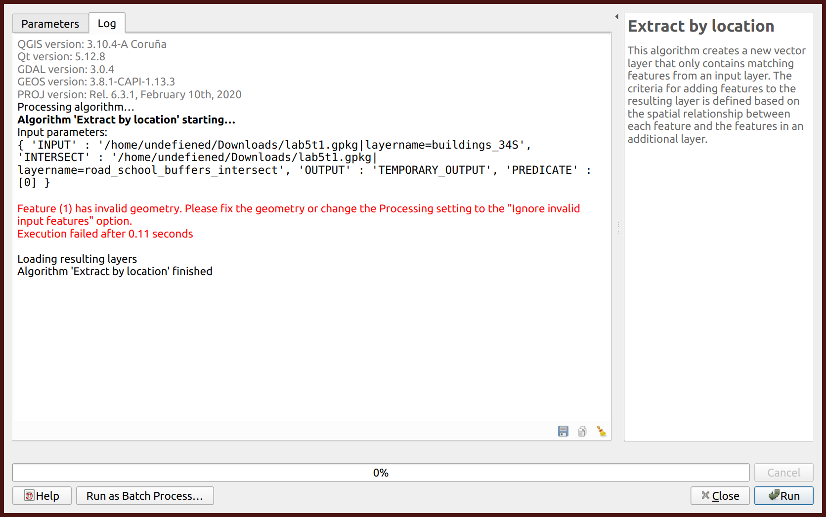
Click Run
You will see that the algorithm reports an error "Feature (1) has invalid geometry. Please fix the geometry or change the Processing setting to the "Ignore invalid input features" option.". That means that the layer buildings_34S has features with problematic geometry. In order to proceed, we need to fix the problematic geometry.
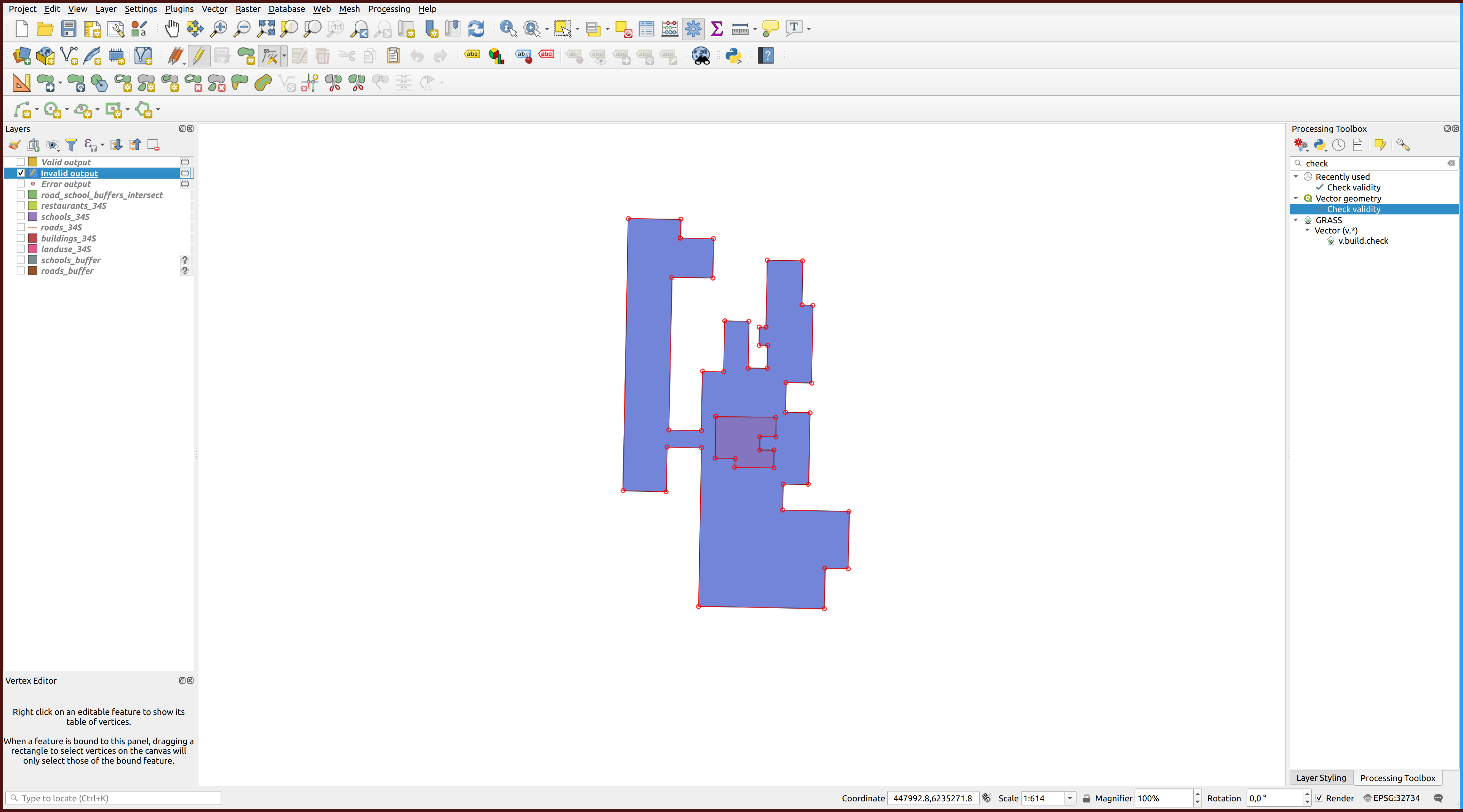
First, let's analyse what features have wrong geometry. Temporarily close Extract by location window. Look for the menu entry Vector geometry ‣ Check validity, select the buildings layer, and run the algorithm.
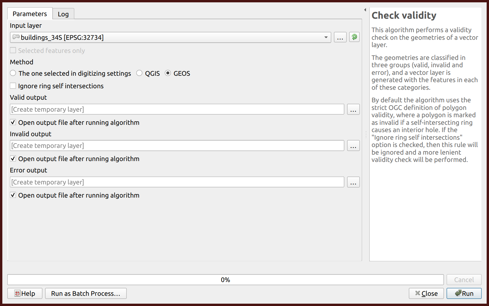
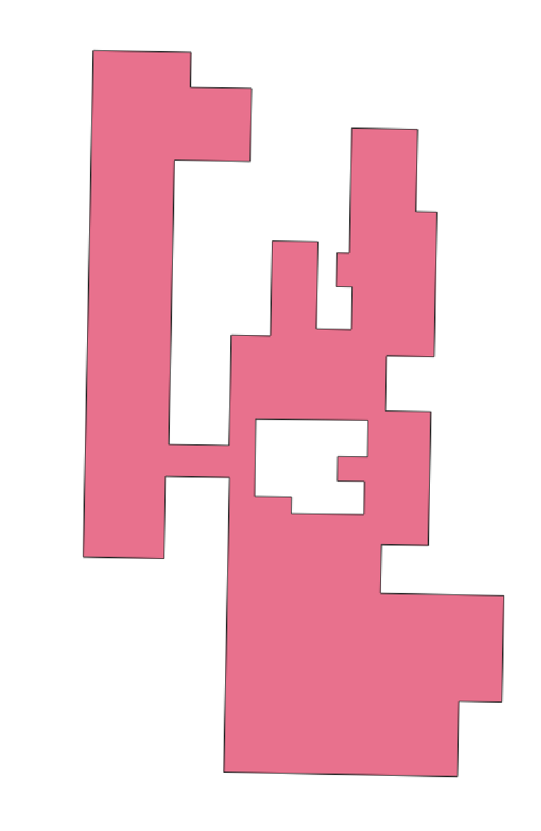
As a result, the algorithm will report that it has found three invalid features and three new layers will appear in the list of layers: Valid output, Invalid output, and Error output.
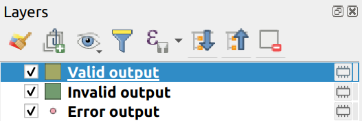
Invalid output is of more importance for us, so remove the other two layers. Invalid output layer contains all features that have invalid geometry. Select some appropriate distinct color for this layer and put it on top to make it visible. There are only two features in this layer, so you can zoom to either of them.
-
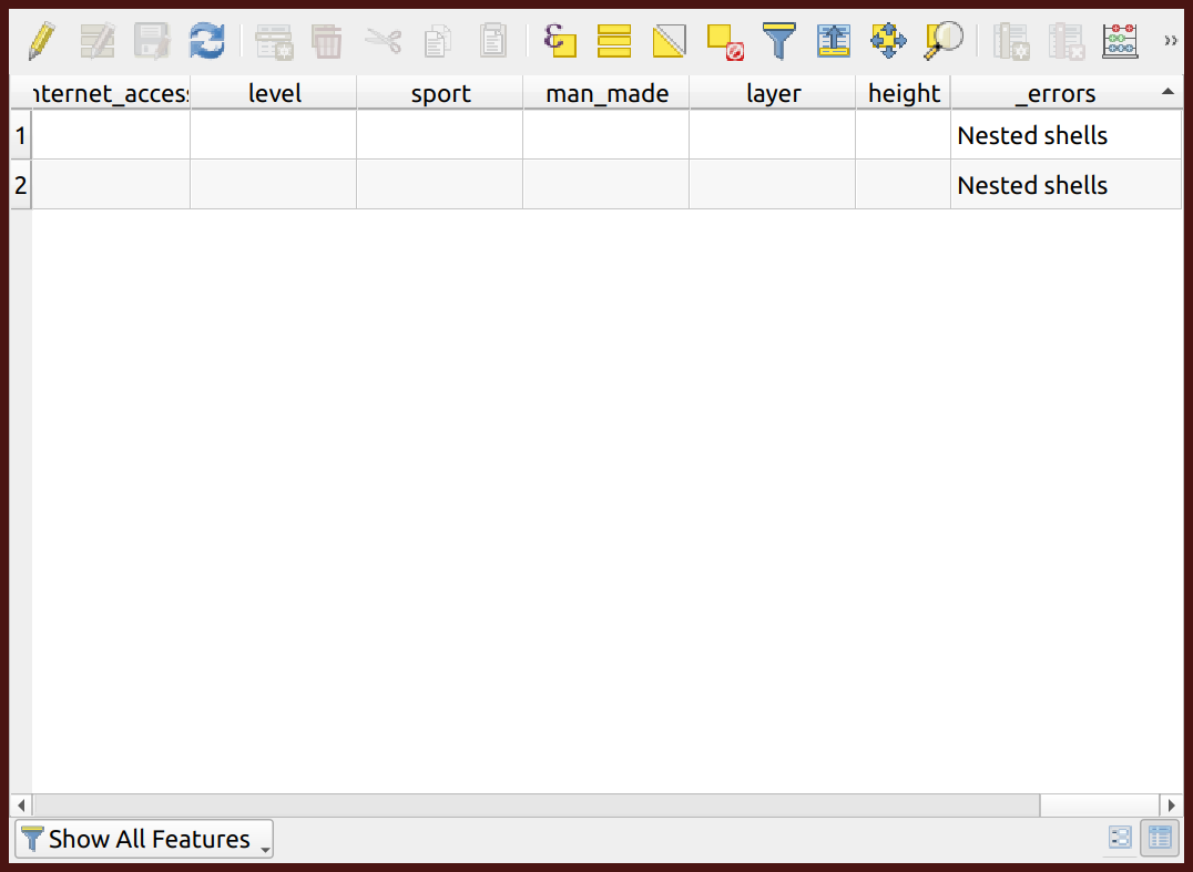
Now, if you will open Attributes table of the Invalid output layer and scroll to the right, you will find a new column in the end with name errors. This is a column added by the Check validity algorithm and it is intended to clarify what is exactly wrong with the geometry. For both of our features it says "Nested shells". This means that one polygon of a multi-polygon feature is completely within another polygon (please note that the buildings layer has multi-polygon geometry type, which means that one feature can consist of several separate polygons).
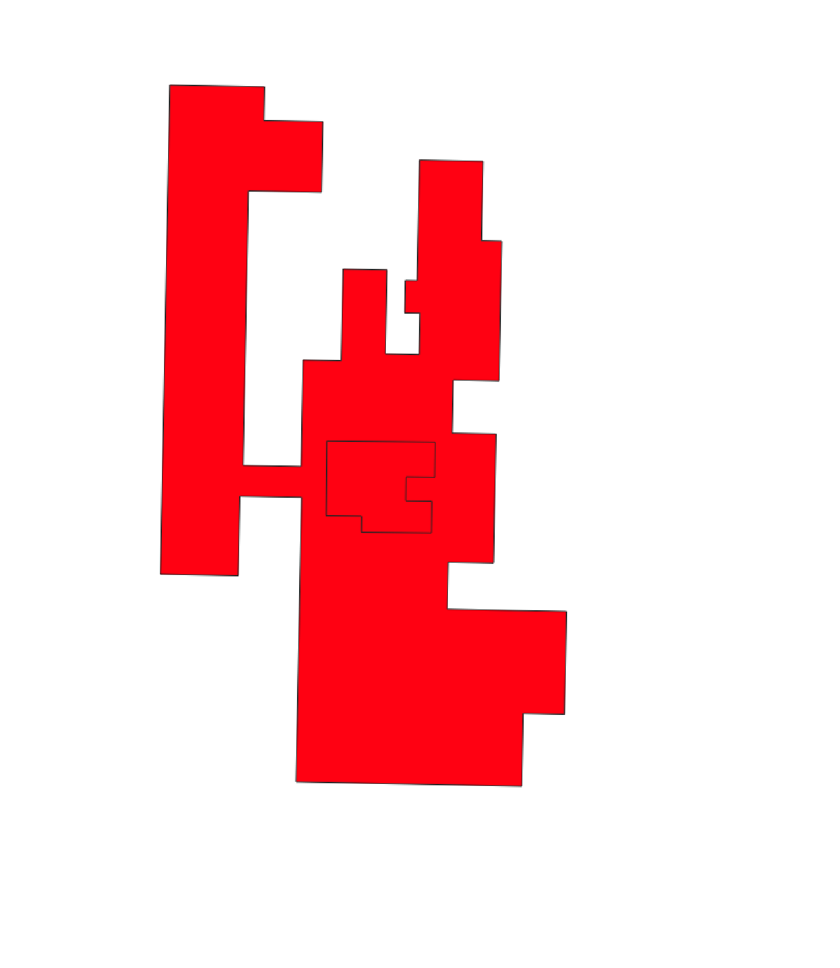
If you enable editing mode and select the feature, you'll probably find that the feature indeed consists of two different polygons: the inner part is completely contained within the outer part.
There are several possibilities of how to fix the invalid geometry. One approach would be to manually remove the inner part or make a hole in the outer part with the shape of the inner part. However, this can be cumbersome if there are many features with invalid geometry. In this scenario, you may use Vector geometry ‣ Fix geometries algorithm that will automatically fix all features with invalid geometry (however, without guarantees that the result will satisfy you). Find the algorithm in the Processing toolbox and set it like in the picture below.
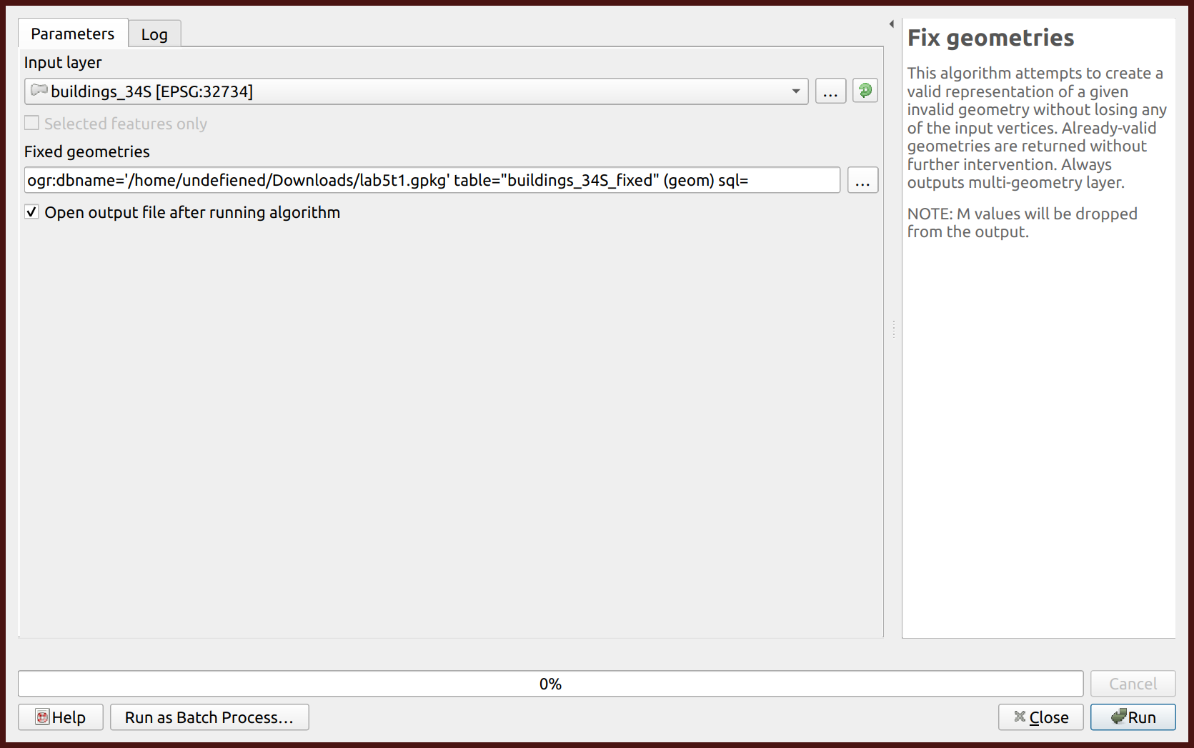
Now, you have a new buildings layer with fixed geometries. If you check, you will find that the Fix geometries algorithm simply cutted holes and removed inner polygons in the features with invalid geometry. While generally this might be not appropriate, for the purpose of our task it is good enough. You can now remove buildings_34S from layer list.
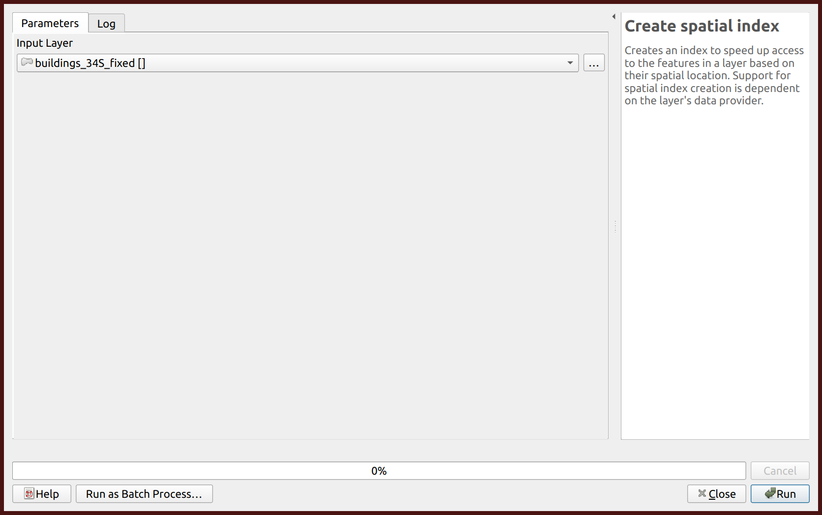
Now you can run Extract by location algorithm again, but this time using the buildings layer with fixed geometry. If you see "No spatial index exists for input layer, performance will be severely degraded", you may go into menu Vector ‣ Data Management Tools ‣ Create Spatial Index..., select the fixed buildings layer in the window and run the algorithm to build the index to improve the speed of QGIS.
After running the Extract by location algorithm again, you’ll probably find that not much seems to have changed. If so, move the well_located_houses layer to the top of the layers list, then zoom in.
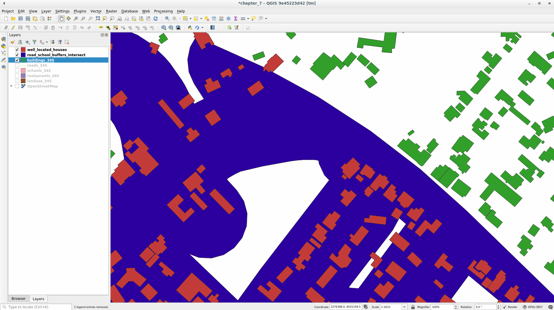
The red buildings are those which match our criteria, while the buildings in green are those which do not.
Now you have two separated layers and can remove buildings_34S_fixed from layer list.
10.  Try Yourself Further Filter our Buildings
We now have a layer which shows us all the buildings within 1km of a school and within 50m of a road. We now need to reduce that selection to only show buildings which are within 500m of a restaurant.
Using the processes described above, create a new layer called houses_restaurants_500m which further filters your well_located_houses layer to show only those which are within 500m of a restaurant.
11. Follow Along: Select Buildings of the Right Size
To see which buildings are of the correct size (more than 100 square meters), we first need to calculate their size.
Select the houses_restaurants_500m layer and open the Field Calculator by clicking on the
 button in
the main toolbar or within the attribute table
button in
the main toolbar or within the attribute tableSet it up like this
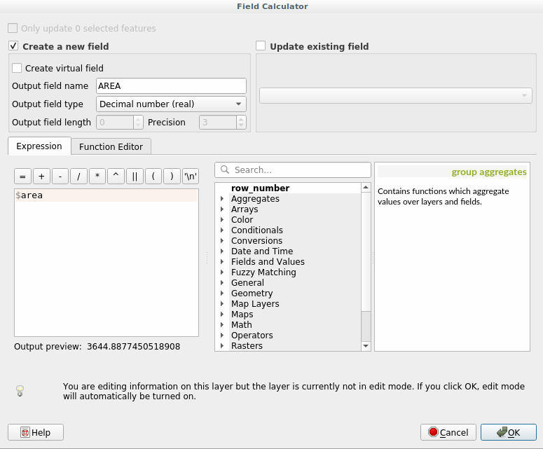
We are creating the new field AREA that will contain the area of each building square meters.
Click OK. The AREA field has been added at the end of the attribute table.
Click the edit mode button again to finish editing, and save your edits when prompted.
Build a query as earlier in this lesson
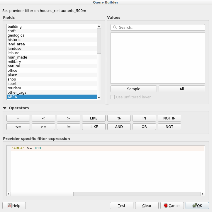
Click OK.

Your map should now only show you those buildings which match our starting criteria and which are more than 100m squared in size.
12. Try Yourself
Save your solution as a new layer, using the approach you learned above for doing so. The file should be saved within the same GeoPackage database, with the name solution.
Tutorial 2: Network Analysis
Calculating the shortest distance between two points is a commonly cited use for GIS. Tools for this can be found in the Processing toolbox.
The goal for this lesson: learn to use Network analysis algorithms.
1.  Follow Along: The Tools and the Data
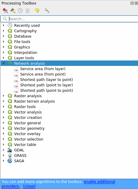
You can find all the network analysis algorithms in the menu. You can see that there are many tools available:
Open the project from this zip-archive, it contains two layers:
- network_points
- network_lines
As you can see the network_lines layer has already a style that helps to understand the road network.
The shortest path tools provide ways to calculate either the shortest or the fastest path between two points of a network, given:
- start point and end point selected on the map
- start point selected on the map and end points taken from a point layer
- start points taken from a point layer and end point selected on the map
Let’s start.
2. Calculate the shortest path (point to point)
The allows you to calculate the shortest distance between two manually selected points on the map.
In this example we will calculate the shortest (not fastest) path between two points.
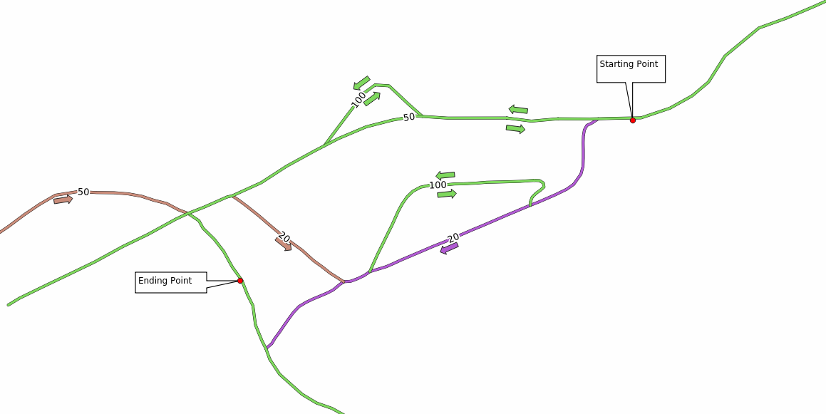
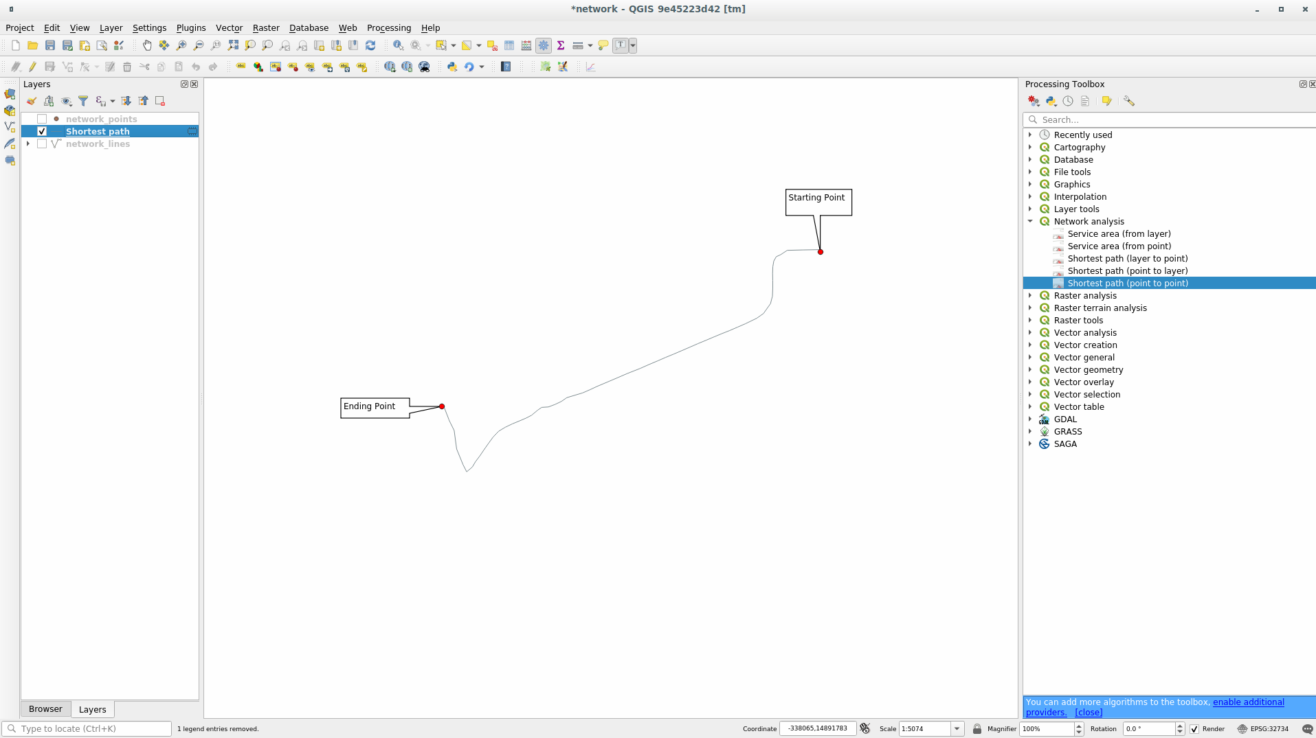
In the following image we choose these two points as starting and ending point for the analysis:
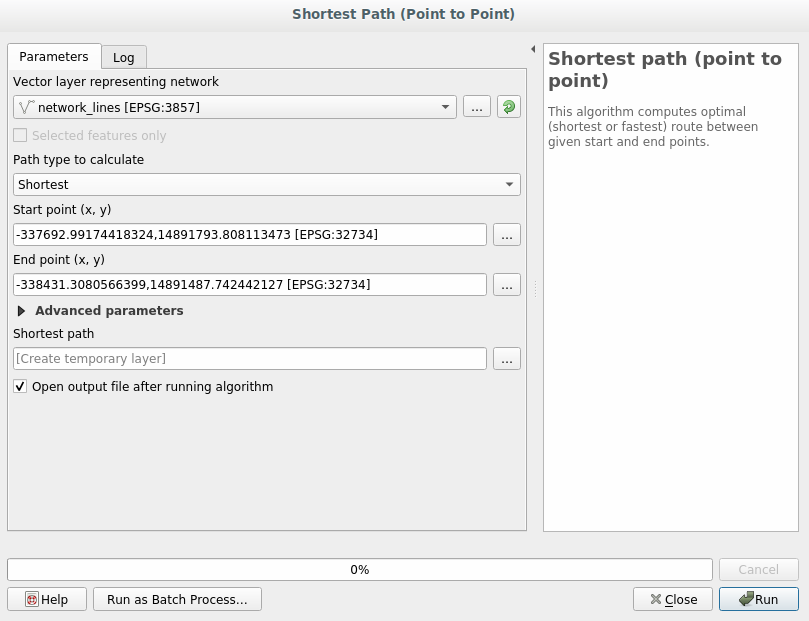
Open the Shortest path (point to point) algorithm
Select network_lines for Vector layer representing network
Let
Shortestin the Path type to calculate parameterClick on the … button next to the Start point (x, y) and choose the location tagged with
Starting Pointin the picture. The menu is filled with the coordinates of the clicked point.Do the same thing but choosing the location tagged with
Ending pointfor End point (x, y)Click on the Run button:
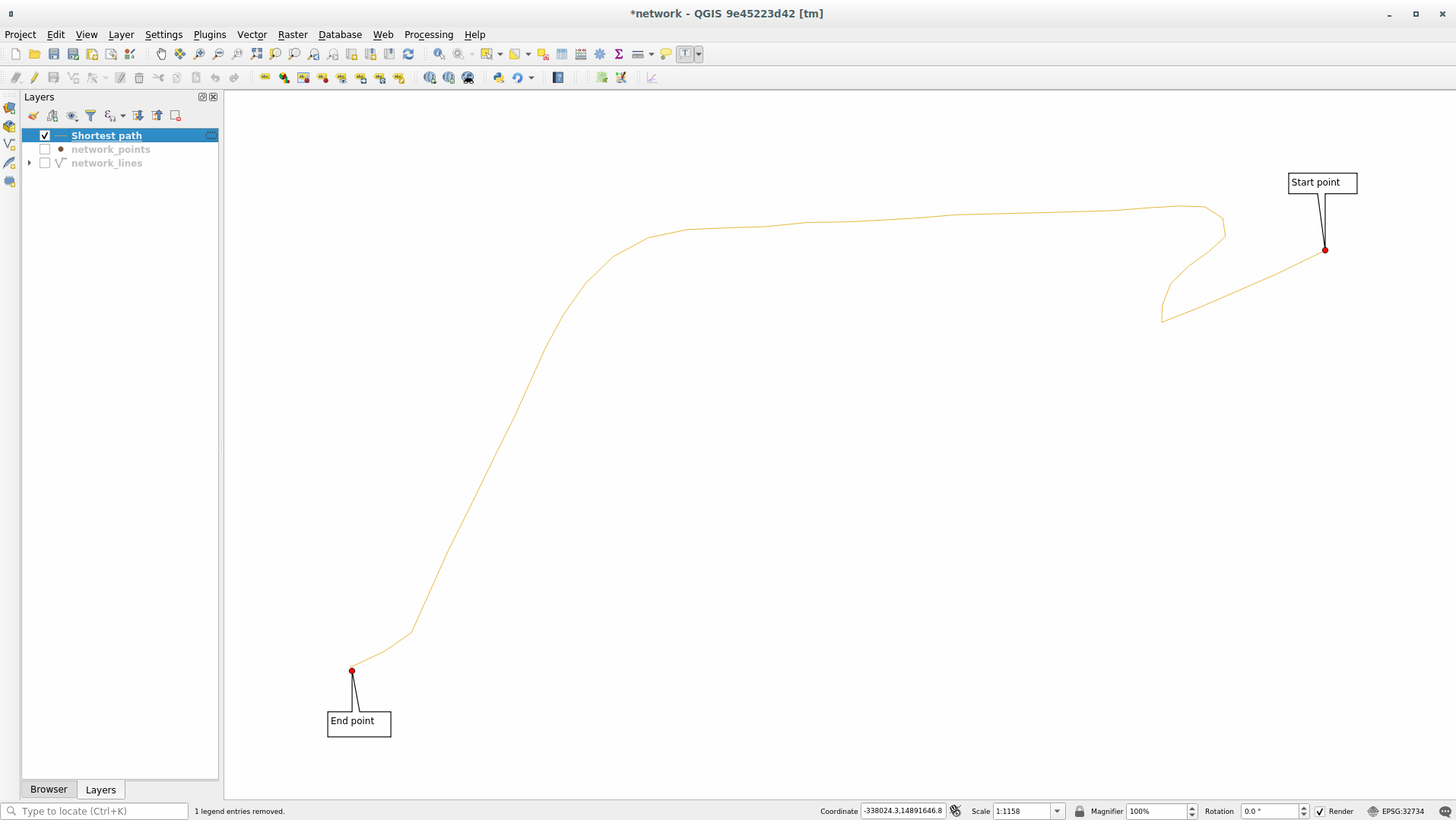
A new line layer is created representing the shortest path between the chosen points. Uncheck the network_lines layer to see the result better:

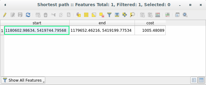
Let’s open the attribute table of the output layer. It contains three fields, representing the coordinates of the starting and ending points and the cost.
We chose
Shortestas Path type to calculate, so the cost represent the distance, in layer units, between the two locations.In our case, the shortest distance between the chosen points is around
1000meters:

Now that you know how to use the tool, feel free to change them and test other locations.
3.  Try Yourself Fastest path
With the same data of the previous exercise, try to calculate the fastest path between the two points.
How much time do you need to go from the start to the end point?
4. Follow Along: Advanced options
Let’s explore some more options of the Network Analysis tools. In the previous exercise we calculated the fastest route between two points. As you can imagine, the time depends on the travel speed.
We will use the same layers and same starting and ending points of the previous exercises.
Open the Shortest path (point to point) algorithm
Fill the Input layer, Start point (x, y) and End point (x, y) as we did before
Choose
Fastestas the Path type to calculateOpen the Advanced parameter menu
Change the Default speed (km/h) from the default
50value to4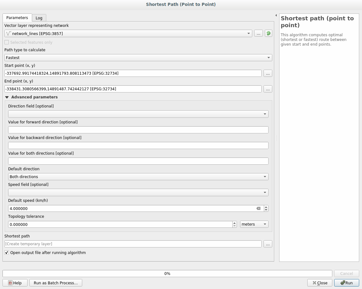
Click on Run
Once the algorithm is finished, close the dialog and open the attribute table of the output layer.
The cost field contains the value according to the speed parameter you have chosen. We can convert the cost field from hours with fractions to the more readable minutes values.
Open the field calculator by clicking on the
 icon and add the
new field minutes by multiplying the cost field by 60:
icon and add the
new field minutes by multiplying the cost field by 60:

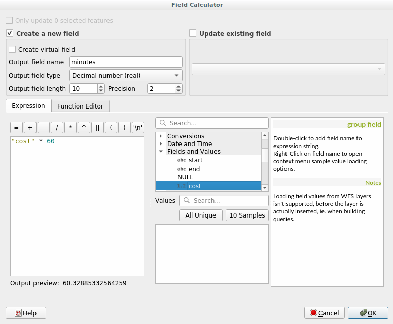
That’s it! Now you know how many minutes it will take to get from one point to the other one.
5.  Shortest map with speed limit
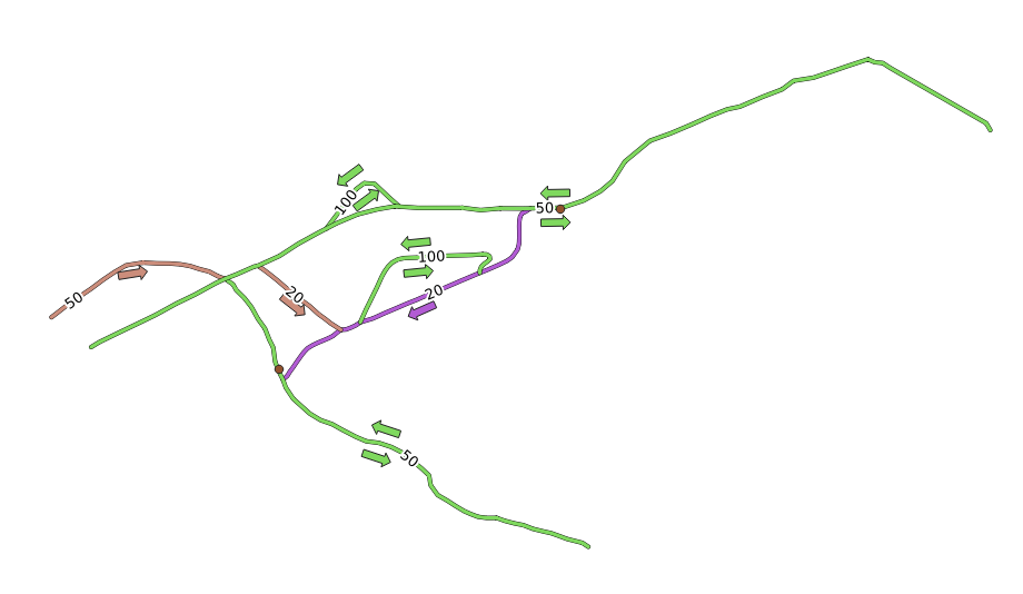
The Network analysis toolbox has other interesting options. Looking at the following map:
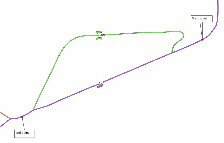
we would like to know the fastest route considering the speed limits of each road (the labels represent the speed limits in km/h). The shortest path without considering speed limits would of course be the purple path. But in that road the speed limit is 20 km/h, while in the green road you can go at 100 km/h!
As we did in the first exercise, we will use the and we will manually choose the start and end points.
Open the algorithm
Select network_lines for the Vector layer representing network parameter
Choose
Fastestas the Path type to calculateClick on the … button next to the Start point (x, y) and choose the location tagged with
Start Pointin the picture. The menu is filled with the coordinates of the clicked point.Do the same thing but choosing the location tagged with
End pointfor End point (x, y)Open the Advanced parameters menu
Choose the
speedfield as the Speed Field parameter. With this option the algorithm will take into account the speed values for each road.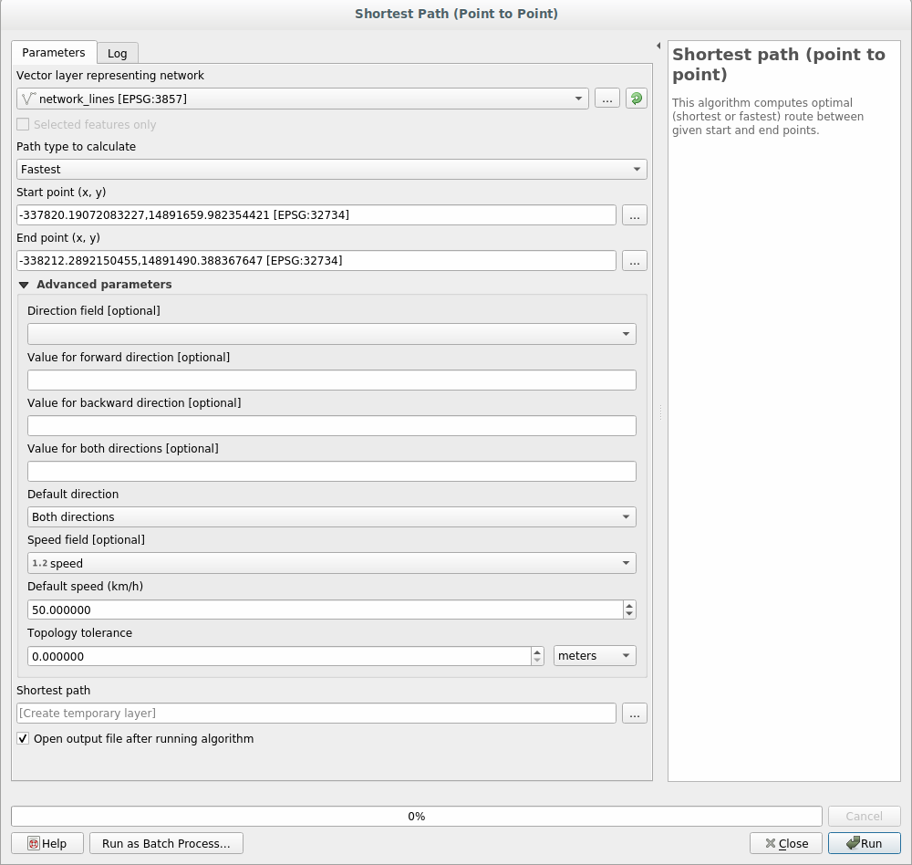
Click on the Run button
Turn off the network_lines layer to better see the result


As you can see the fastest route does not correspond to the shortest one.
6. Service area (from layer)
The algorithm can answer the question: given a point layer, what are all the reachable areas given a distance or a time value?
Note
The is the same algorithm but, it allows you to manually choose the point on the map.
Given a distance of 250 meters we want to know how far we can go on the
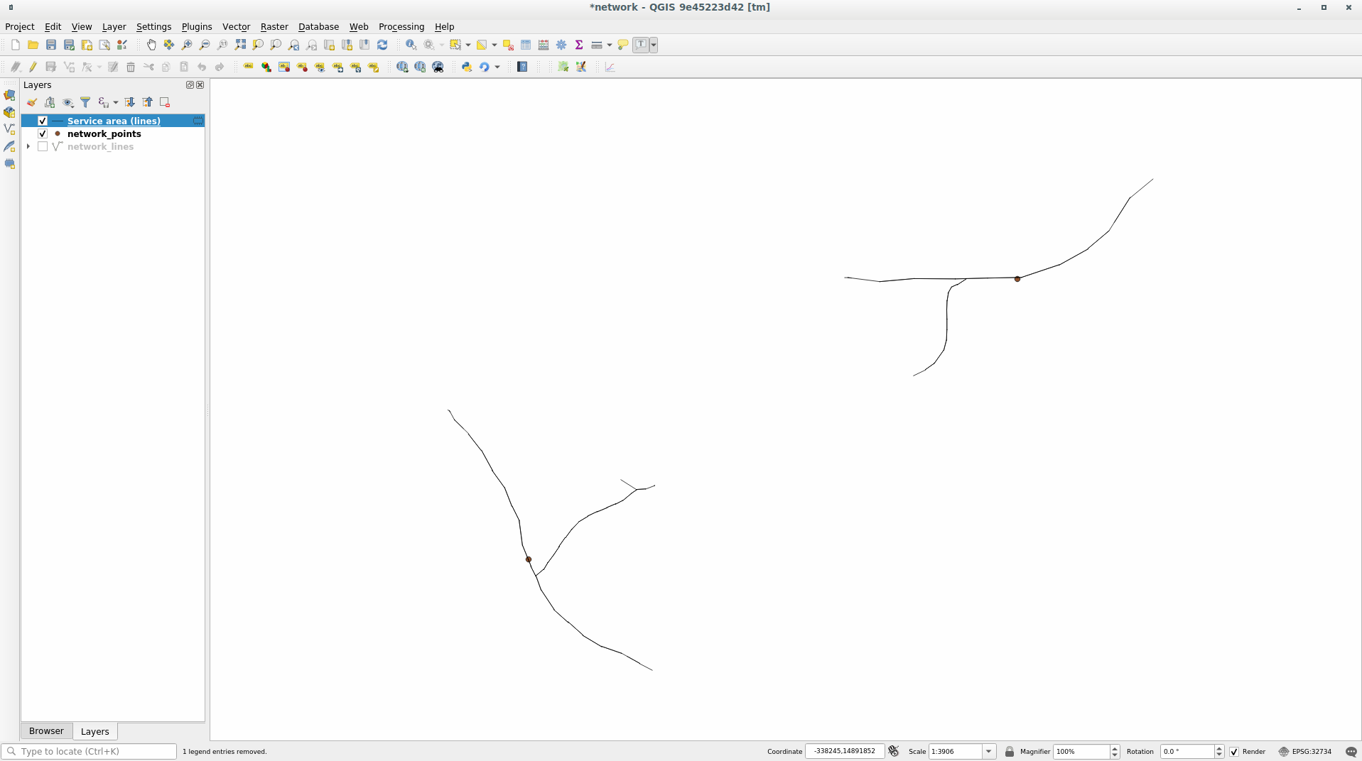
network from each point of the network_points layer.
Uncheck all the layers except network_points
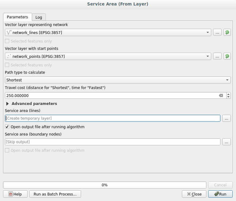
Open the algorithm
Choose network_lines for Vector layer representing network
Choose network_points for Vector layer with start points
Choose
Shortestin Path type to calculateEnter
250in the Travel cost parameterClick on Run and then close the dialog

The output layer represents the maximum path you can reach from the point features given a distance of 250 meters:

Nearest Neighbor Analysis (QGIS3)
GIS is very useful in analyzing spatial relationship between features. One such analysis is finding out which features are closest to a given feature. There are multiple ways to do this analysis in QGIS. In this tutorial,we will explore the Distance to nearest hub and Distance matrix tools to carry out the nearest neighbor analysis.
Overview of the task
Given the locations of all known significant earthquakes, find out the nearest populated place for each location where the earthquake happened.
Other skills you will learn
- Use the Geometry Generator renderer to dynamically create lines from a multipoint layer.
Get the data
We will use NOAA’s National Geophysical Data Center’s Significant Earthquake Database as our layer representing all major earthquakes. Download the tab-delimited earthquake data.
Natural Earth has a nice Populated Places dataset. Download the simple (less columns) dataset
For convenience, you may directly download a copy of both the datasets from the links below:
ne_10m_populated_places_simple.zip
Data Sources: [NGDC] [NATURALEARTH]
Procedure
- Locate the downloaded
ne_10m_populated_places_simple.zipfile in the Browser panel and expand it. Drag thene_10m_populated_places_simple.shpfile to the canvas.
%20%E2%80%94%20QGIS%20Tutorials%20and%20Tips_files/180.png)
- You will see a new layer
ne_10m_populated_places_simpleloaded in the Layers panel. This layer contains the points representing populated places. Now we will load the earthquakes layer. This layer comes as a Tab Serepated Values (TSV) text file. To load this file, click the Open Data Source Manager button on the Data Source Toolbar. You can also useCtrl + Lkeyboard shortcut.
%20%E2%80%94%20QGIS%20Tutorials%20and%20Tips_files/240.png)
- Click the ... button next to File name and browse to the downloaded
signif.txtfile. Once loaded, the File Format and Geometry Definition fields should be auto-populated with correct values. Click Add followed by Close.
%20%E2%80%94%20QGIS%20Tutorials%20and%20Tips_files/329.png)
- Zoom around and explore both the datasets. Each yellow point represents the location of a significant earthquake and each red point represents the location of a populated place. Our goal is to find out the nearest point from the populated places layer for each of the points in the earthquake layer.
%20%E2%80%94%20QGIS%20Tutorials%20and%20Tips_files/415.png)
- Before we do the analysis, we need to clean up our inputs. The
signiflayer contains many records without a valid geometry. These records were imported with a NULL geometry. So let’s remove these records first. Go to .
%20%E2%80%94%20QGIS%20Tutorials%20and%20Tips_files/515.png)
- Search for and locate the tool. Double-click to launch it.
%20%E2%80%94%20QGIS%20Tutorials%20and%20Tips_files/615.png)
- Select
signifas the Input layer and click Run. Once the processing finishes, click Close.
%20%E2%80%94%20QGIS%20Tutorials%20and%20Tips_files/714.png)
- You will see a new layer caled
Non null geometriesloaded into the Layers panel. We will use this layer instead of the originalsigniflayer in further analysis. Un-check thesigniflayer in the Layers panel to hide it. Now it is time to perform the nearest neighbor analysis. Search and locate the tool. Double-click to launch it.
%20%E2%80%94%20QGIS%20Tutorials%20and%20Tips_files/814.png)
Note
If you need point layer as output, use the Distance to nearest hub (points) tool instead.
- In the Distance to Nearest Hub (Line to Hub) dialog, select
Non null geometriesas the Source points layer. Selectne_10m_populated_places_simpleas the Distination hubs layer. Selectnameas the Hub layer name attribute. The tool will also compute straight-line distance between the populated place and the nearest earthquake. SetKilometersas the Measurement unit. Click Run. Once the processing finishes, click Close.
%20%E2%80%94%20QGIS%20Tutorials%20and%20Tips_files/914.png)
- Back in the main QGIS window, you will see a new line layer called
Hub distanceloaded in the Layers panel. This layer has line features connecting each earthquake point to the nearest populated place. Right-click theHub distancelayer and select Open Attribute Table.
%20%E2%80%94%20QGIS%20Tutorials%20and%20Tips_files/1014.png)
- Scroll right to the last columns and you will see 2 new attributes called HubName and HubDist added to the original earthquake features. This is the name the distance to the nearest neighbor from the populated places layer.
%20%E2%80%94%20QGIS%20Tutorials%20and%20Tips_files/1117.png)
- Our analysis is complete. We can now explore another tool that can also do a similar analysis. Distance Matrix
is a powerful tool that allows you to not only compute distance to the
nearest point, but to all the points from another layer. We can use this
method as an alternative to the Distance to nearest hub tool. Un-check the
Hub distancelayer to hide it. Search and locate the tool.
%20%E2%80%94%20QGIS%20Tutorials%20and%20Tips_files/1215.png)
- In the Distance matrix dialog, set
Non null geometriesas the Input point laeyer andI_Das the Input unique ID field. Setne_10m_populated_places_simpleas the Target point layer andnameas the Target unique ID field. SelectLinear (N*k x 3) distance matrixas the Output matrix type. The key here is to set the Use only the nearest (k) target points parameter to1- which will give you only the nearest neighbor in the output. Click Run to start the matrix calculation. Once the processing finishes, click Close.
%20%E2%80%94%20QGIS%20Tutorials%20and%20Tips_files/1315.png)
- Once the processing finishes, a new layer called
Distance matrixwill be loaded. Note that the output of this tool is a layer containin MultiPoint geometries. Each feature contains 2 points - source and target. Open the Attribute Table for the layer. You will see that each feature has attributes mapping the earthquake to its nearest populated place. Note that the distance here is in the layer’s CRS units (degrees).
%20%E2%80%94%20QGIS%20Tutorials%20and%20Tips_files/1413.png)
- At this point, you can save your results in the format of your choice by right-clicking the layer and selecting .
If you want to visualize the results better, we can easily create a
hub-spoke rendering from the feature’s geometry. Right-click the
Distance matrixlayer and select Properties.
%20%E2%80%94%20QGIS%20Tutorials%20and%20Tips_files/1512.png)
- In the Properties dialog, switch to the Symbology tab. Click on the
Simple markersub-renderer and selectGeometry generatoras the Symbol layer type. SetLineString / MultiLineStringas the Geometry type. Click the Expression button.
%20%E2%80%94%20QGIS%20Tutorials%20and%20Tips_files/1612.png)
- Here we can enter an expression to create a line geometry from the 2 points within each multi-point source geometry. Enter the following expression.
make_line(point_n( $geometry, 1), point_n( $geometry, 2))%20%E2%80%94%20QGIS%20Tutorials%20and%20Tips_files/1712.png)
- Back in the Symbology tab, set the style of the line as per your liking and click OK.
%20%E2%80%94%20QGIS%20Tutorials%20and%20Tips_files/1811.png)
- You will see the
Distance matrixlayer now rendered with lines instead of points. Note that we did not have to create a new layer for this visualization. The layer still contains MultiPoint geometries, but it is dynamically rendered as lines based on the expression.
%20%E2%80%94%20QGIS%20Tutorials%20and%20Tips_files/1910.png)
Assignment
Hazardous material (HazMat) like gasoline, ammonium, propane, etc is frequently transported through populated areas. In order to reduce the risk for life and property there are restrictions for the building of houses near main transport routes. According to these no building at all should be located closer that 25 meters from the side of a road where hazmat is frequently transported. Buildings where several people work or spend time daily should have at least 40 meters distance to the road side and dwelling houses (where people sleep at night) should be located at least 75 m from the roadside
Launch QGIS and create a new map using the data from this GeoPackage file. Select "SWEREF99/RT90 2.5 gon V emulation" CRS for the project and for all layers (please refer to instruction in the Lab 1 assignment). There are two different possibilities to guide hazmat-transports from north to south-east through Norrköping. These are marked as route 1 and 2. Your task is to find out which route is the best alternative considering the risk distances mentioned above. You should give a motivation to your choice in the conclusion of the report.
The demography layer shows the number of people that live in each parcel (piece of land). The point shows the centroids (centrally located points) of all parcels and the table connected to the points shows the total number of people and their distribution on age classes. You can for instance calculate the number of school children in an arbitrary area by this data.
The routes show centrelines of the streets. When you calculate the number of objects that are within a certain distance you must therefore add 5 meters to the distances given above. Use the Vector Selection > Extract by location tool in the processing toolbox to extract necessary features to a separate layer and use this layer to compute the number of buildings or people affected.
| Route | Number of buildings partly within 25 m from the roadside | Number of buildings completely within 40 m from the roadside | Number of persons living within 75 m from the roadside |
| 1 | |||
| 2 |
Use the values you calculate to fill out the table above, copy and insert it in the report.
The report shall also be attached by a layout with a map that shows the routes and the outlines of an 80-meter buffer zone (on each side) along each route. The layers landuse, streets and buildings should be visible on the map.
Tutorial 3 is a courtesy of QGIS tutorial by Ujaval Gandhi and shared here in accordance with CC-BY 4.0 license under the same license. Thank you, Ujaval Gandhi!