Lab 4 Tutorial 1 Tutorial 2 Tutorial 3 Tutorial 4 Assignment <-- Back to the course page

Tutorial 1: Digitizing Map Data¶

Digitizing is one of the most common tasks that a GIS Specialist has to do. Often a large amount of GIS time is spent in digitizing raster data to create vector layers that you use in your analysis. QGIS has powerful on-screen digitizing and editing capabilities that we will explore in this tutorial.

Overview of the task¶

We will use a raster topographic map and create several vector layers representing features around a park.

Other skills you will learn¶

Building pyramids for large raster datasets to speed up zoom and pan operations.
Working with a Spatialite database.

Get the data¶

Land Information New Zealand (LINZ) provides raster topographic maps at 1:50,000 scale for the New Zealand mainland and Chatham Islands.

Download the GeoTIFF Image file from the Christchurch Topo50 map download page.

For convenience, you may directly download a copy of the dataset from the link below:

BX24_GeoTifv1-02-clip.tif

Data Source [LINZ]

Procedure¶

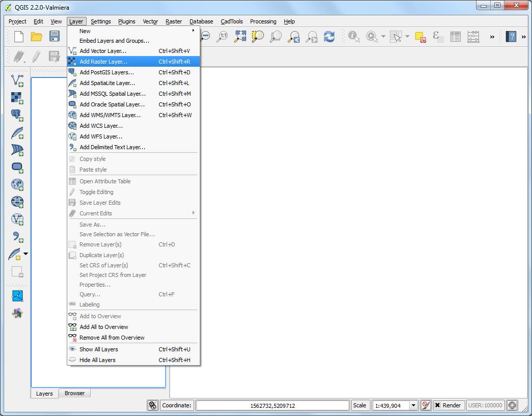
Go to Layer ‣ Add Raster Layer. Locate the downloaded BX24_GeoTifv1-02.tif and click Open.

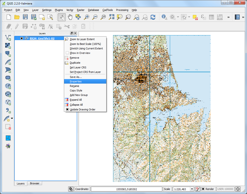
This is a large raster file and you may notice that when you zoom or pan around the map, the map takes a little time to render the image. QGIS offers a simple solution to make rasters load much faster by using Image Pyramids. QGIS creates pre-rendered tiles at different resolutions and these are presented to you instead of the full raster. This makes map navigation snappy and responsive. Right-click the BX24_GeoTifv1-02 layer and choose Properties.

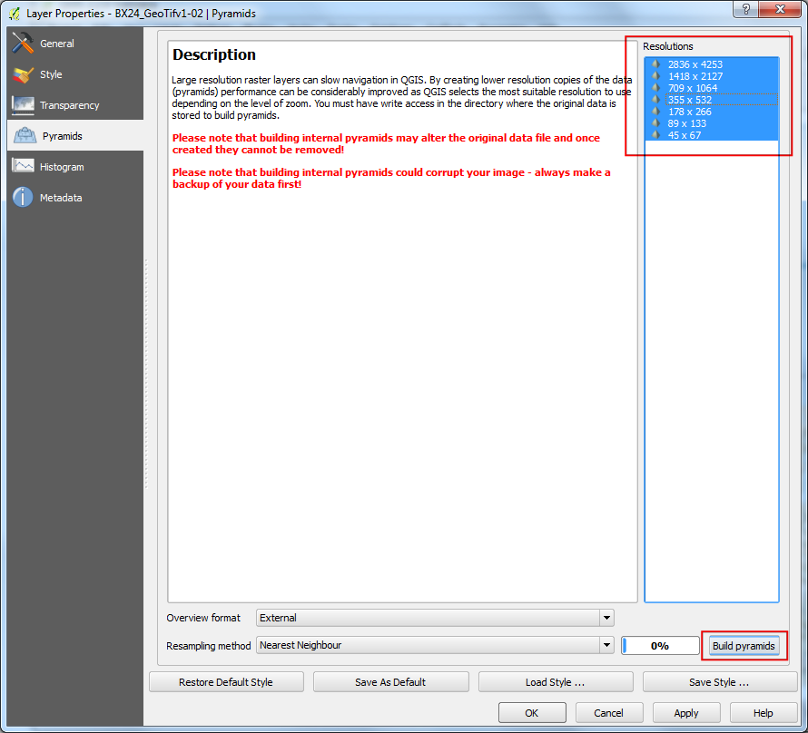
Choose the Pyramids tab. Hold the Ctrl key and select all the resolutios offered in the Resolutions panel. Leave other options to defaults and click Build pyramids. Once the process finishes, click OK.

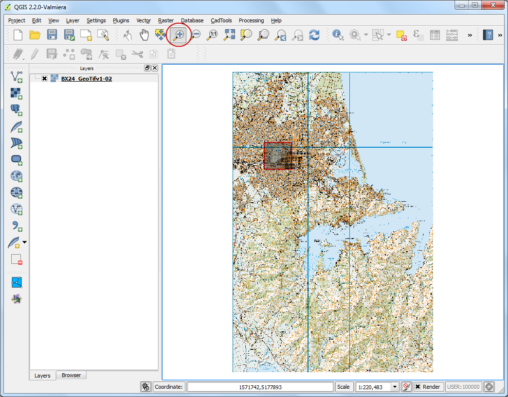
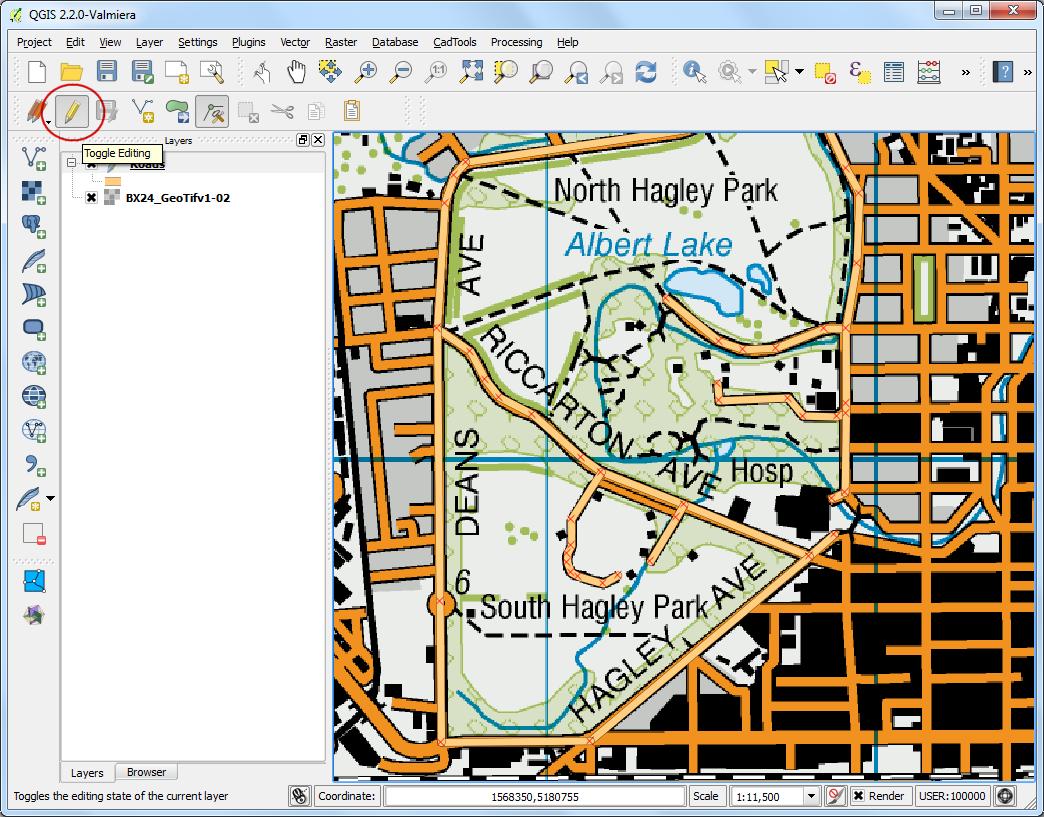
Back in the main QGIS window, use the Zoom tool to locate Hagley Park area in Christchurch. This is the park that we will be digitizing.

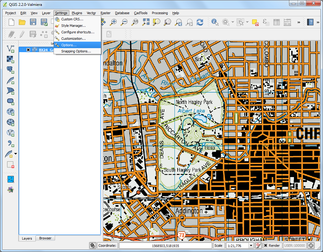
Before we start, we need to set default Digitizing Options. Go to Settings ‣ Options....

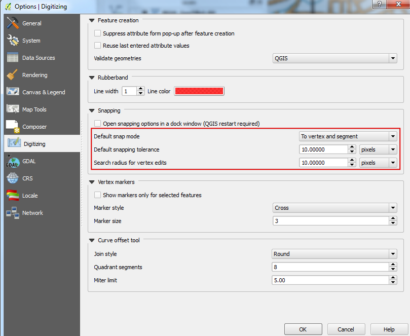
Select the Digitizing tab in the Options dialog. Set the Default snap mode to To vertex and segment. This will allow you to snap to the nearest vertex or line segment. I also prefer to set the Default snapping tolerance and Search radius for vertex edits in pixels instead of map units. This will ensure that the snapping distance remains constant regardless of zoom level. Depending on your computer screen resolution, you may choose an appropriate value. Click OK.

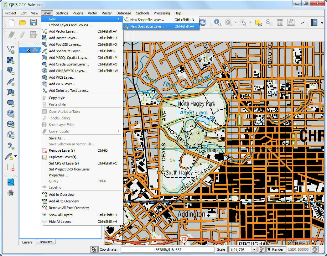
Now we are ready to start digitizing. We will first create a roads layer and digitize the roads around the park area. Select Layer ‣ New ‣ New Spatialite Layer.... You may also choose to create a New Shapefile Layer... instead if you prefer. Spatialite is an open database format similar to ESRI’s geodatabase format. Spatialite database is contained within a single file on your hard drive and can contain diferent types of spatial (point, line, polygon) as well as non-spatial layers. This makes is much easier to move it around instead of a bunch of shapefiles. In this tutorial, we are creating a couple of polygon layers and a line layer, so a Spatialite database will be better suited. You can always load a spatialite layer and save it as a shapefile or any other format you want.

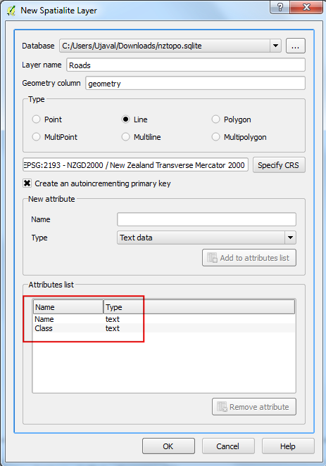
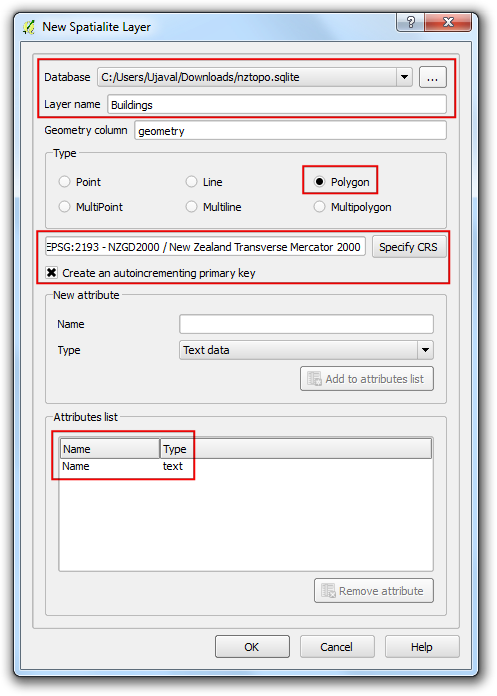
In the New Spatialite Layer dialog, click the ... button and save a new spatialite database named nztopo.sqlite. Choose the Layer name as Roads and select Line as the Type. The base topographic map is in the EPSG:2193 - NZGD 2000 CRS, so we can select the same for our roads layer. Check the Create an autoincrementing primary key box. This will create a field called pkuid in the attribute table and assign a unique numeric id automatically to each feature. When creating a GIS layer, you must decide on the attributes that each feature will have. Since this is a roads layer, we will have 2 basic attributes - Name and Class. Enter Name as the Name of the attribute in the New attribute section and click Add to attribute list.

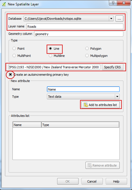
Similarly create a new attribute Class of the type Text data. Click OK.

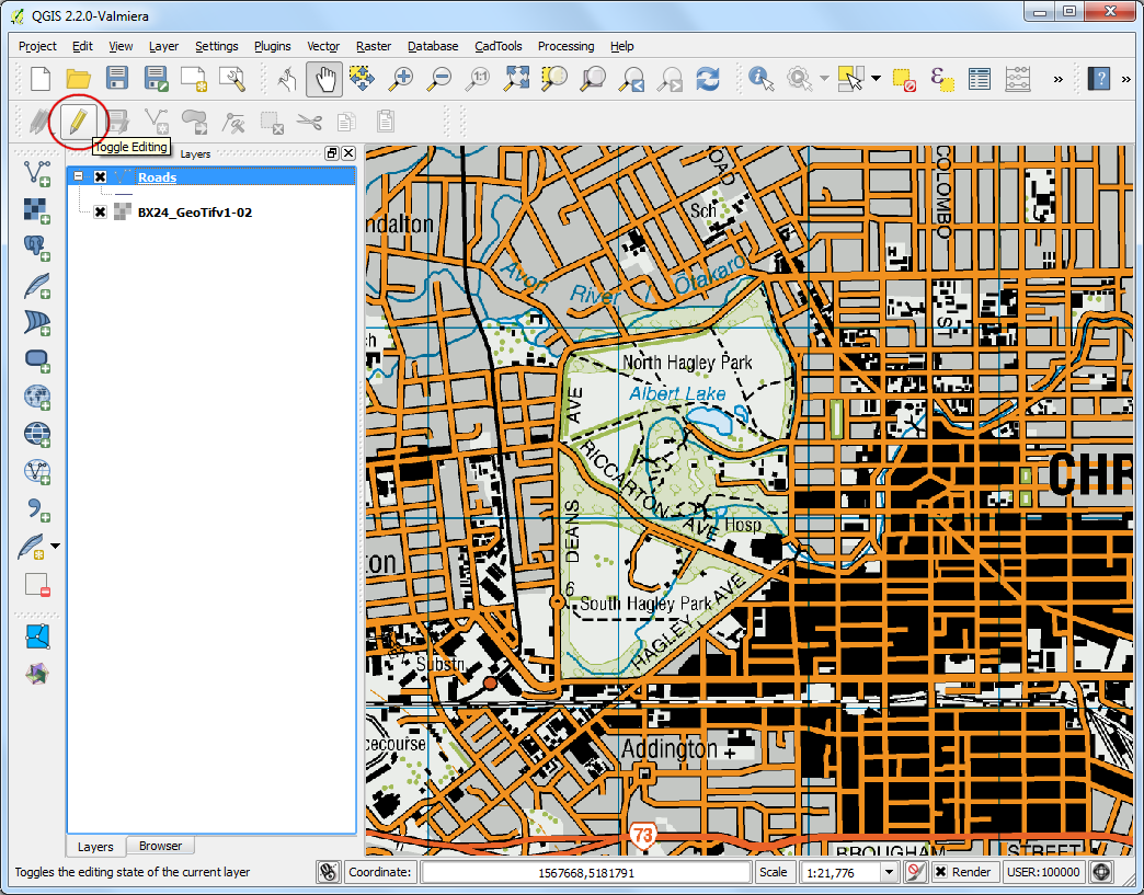
Once the layer is loaded, click the Toggle Editing button to put the layer in editing mode.

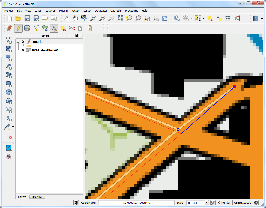
Click the Add feature button. Click on the map canvas to add a new vertex. Add new vertices along the road feature. Once you have digitized a road segment, right-click to end the feature.

Note

You can use the scroll wheel of the mouse to zoom in or out while digitizing. You can also hold the scroll button and move the mouse to pan around.

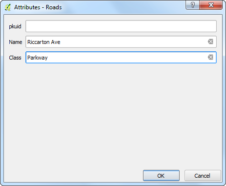
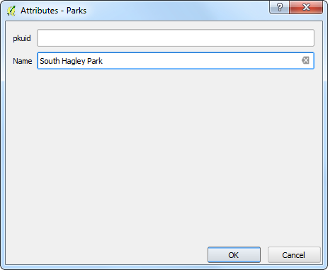
After you right-click to end the feature, you will get a pop-up dialog called Attributes. Here you can enter attributes of the newly created feature. Since the pkuid is an auto-incrementing field, you will not be able to enter a value manually. Leave it blank and enter the road name as it appears on the topo map. Optionally, assign a Road Class value as well. Click OK.

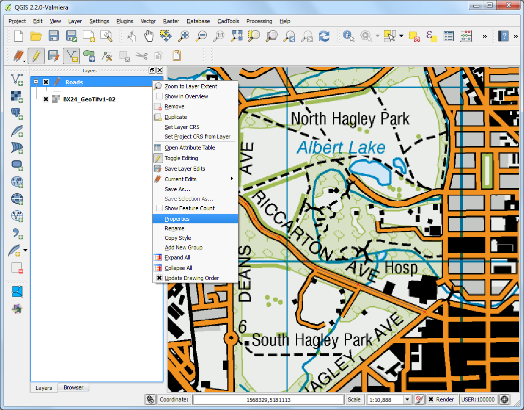
The default style of the new line layer is a thin line. Let’s change it so we can better see the digitized features on the canvas. Right click the Roads layer and select Properties.

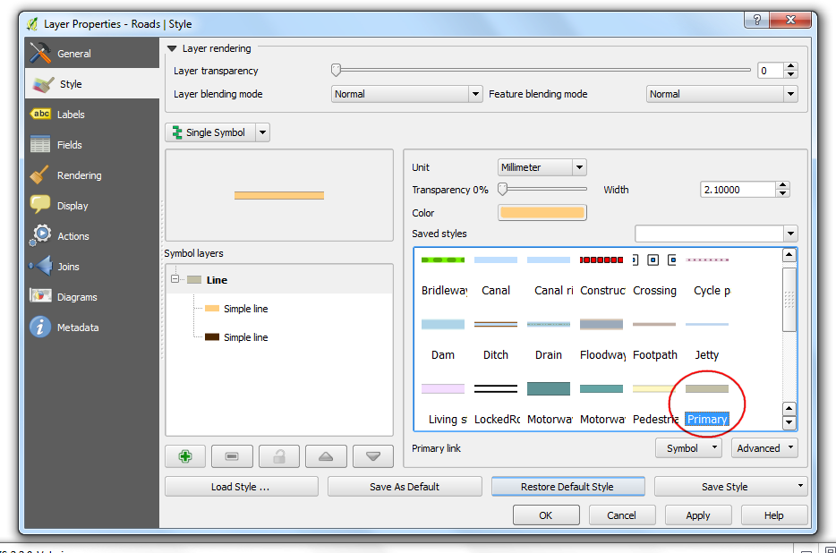
Select the Style tab in the Layer Properties dialog. Choose a thicker line style such as Primary from the predefined styles. Click OK.

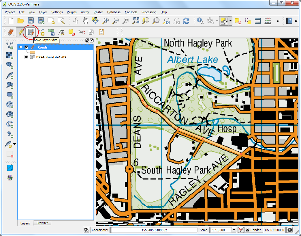
Now you will see the digitized road feature clearly. Click Save Layer Edits to commit the new feature to disk.

Before we digitize remaining roads, it is important to update some other settings that are important to create an error free layer. Go to Project ‣ Snapping Options.

In the dialog enable snapping by clicking on the Enable snapping button. Then check the Topological editing. This option will ensure that the common boundaries are maintained correctly in polygon layers. Also check the Snapping on intersection which allows you to snap on an intersection of a background layer.

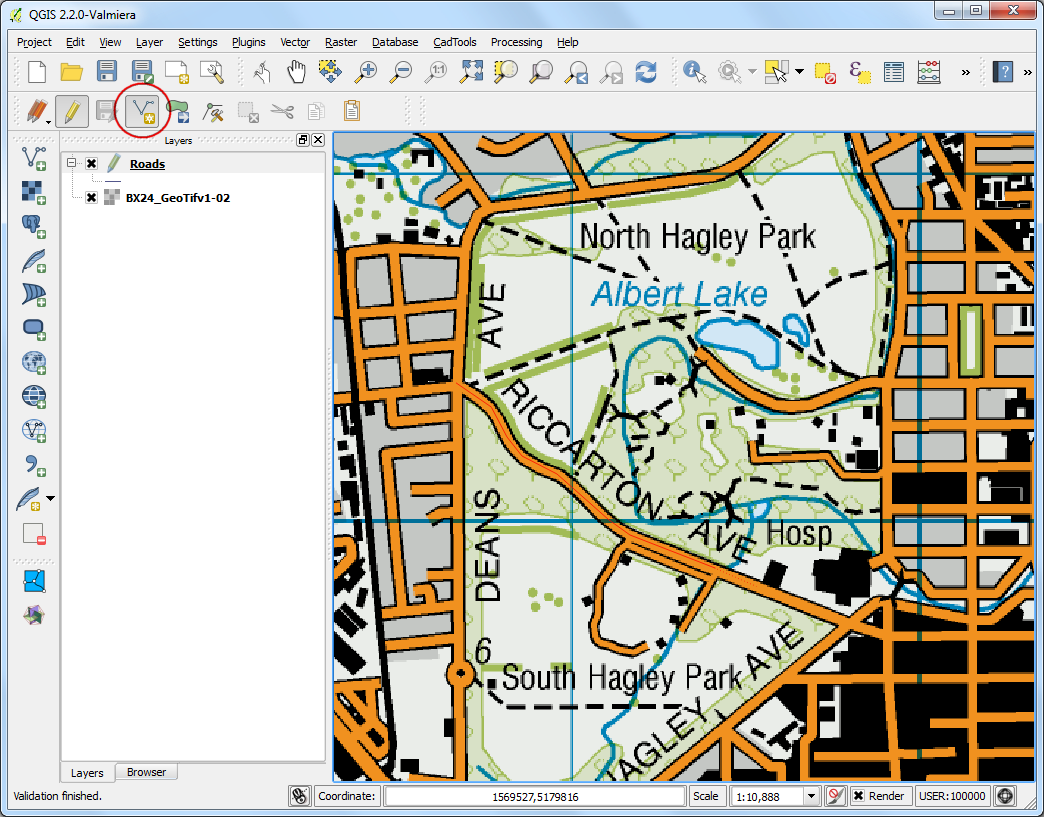
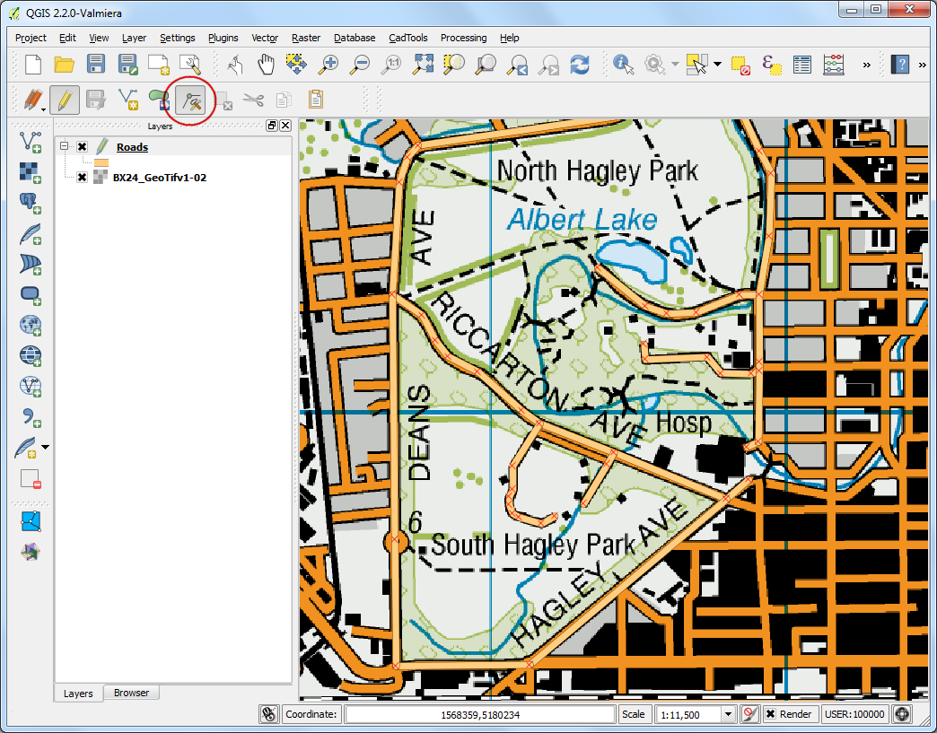
Now you can click Add feature button and digitize other roads around the park. Make sure to click Save Edits after you add a new feaure to save your work. A useful tool to help you with digitizing is the Vertex Tool. Click the Vertex Tool button.

Once the vertex tool is activated, click on any feature to show the vertices. Click on any vertex to select it. The vertex will change the color once it is selected. Now you can click and drag your mouse to move the vertex. This is useful when you want to make adjustments after the feature is created. You can also delete a selected vertex by clicking the Delete key. (Option+Delete on a mac)

Once you have finished digitizing all the roads, click the Toggle Editing button.

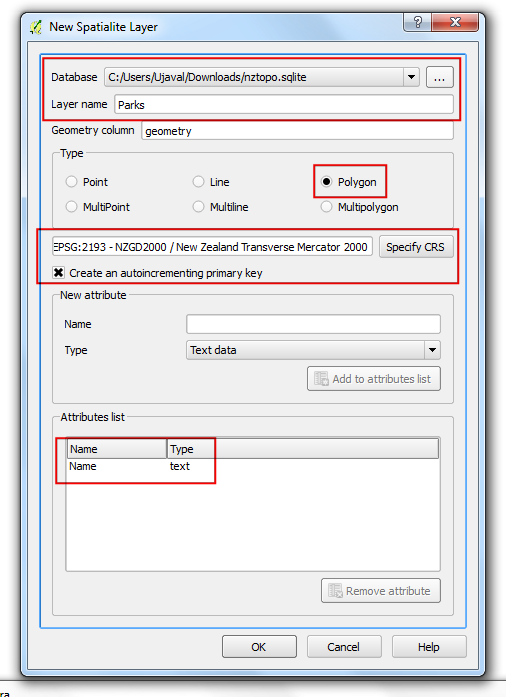
Now we will create a polygon layer representing the park boundaries. Go to Layer ‣ New ‣ New Spatialite Layer.... Select the nztopo.sqlite database from the dropdown list. Name the new layer as Parks. Select Polygon as the Type. Create a new attribute called Name. Click OK.

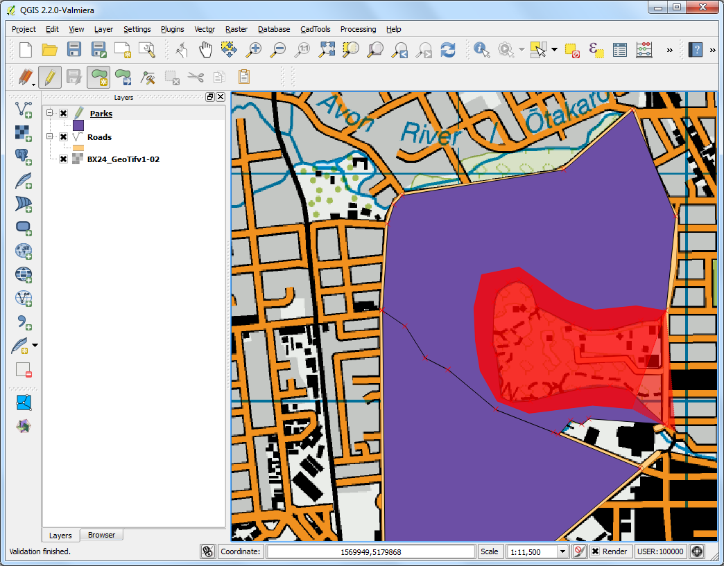
Click the Add feature button and click on the map canvas to add a polygon vertex. Digitize the polygon representing the park. Make sure you snap to the roads vertices so there are no gaps between the park polygons and road lines. Right-click to finish the polygon.

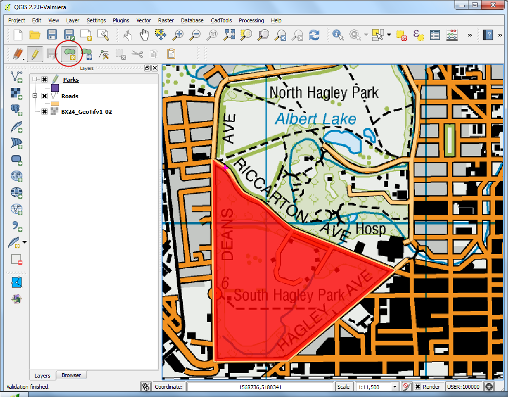
Enter the park name in the Attributes pop-up.

Polygon layers offer another very useful setting called Avoid Overlap on Active Layer. Go to Project ‣ Snapping Options. Click on the button Allow overlap and select the value Avoid Overlap on Active Layer.

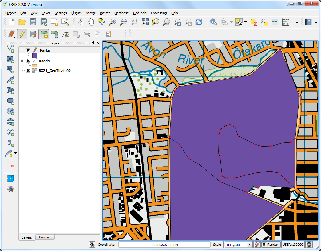
Now click on Add feature to add a polygon. With the Avoid Overlap on Active Layer, you will be able quickly digitize a new polygon without worrying about snapping exactly to the neighboring polygons.

Right-click to finish the polygon and enter the attributes. Magically the new polygon is shrunk and snapped exactly to the boundary of the neighboring polygons! This is very useful when digitizing complex boundaries where you need not be very precise and still have topologically correct polygon. Click Toggle Editing to finish editing the Parks layer.

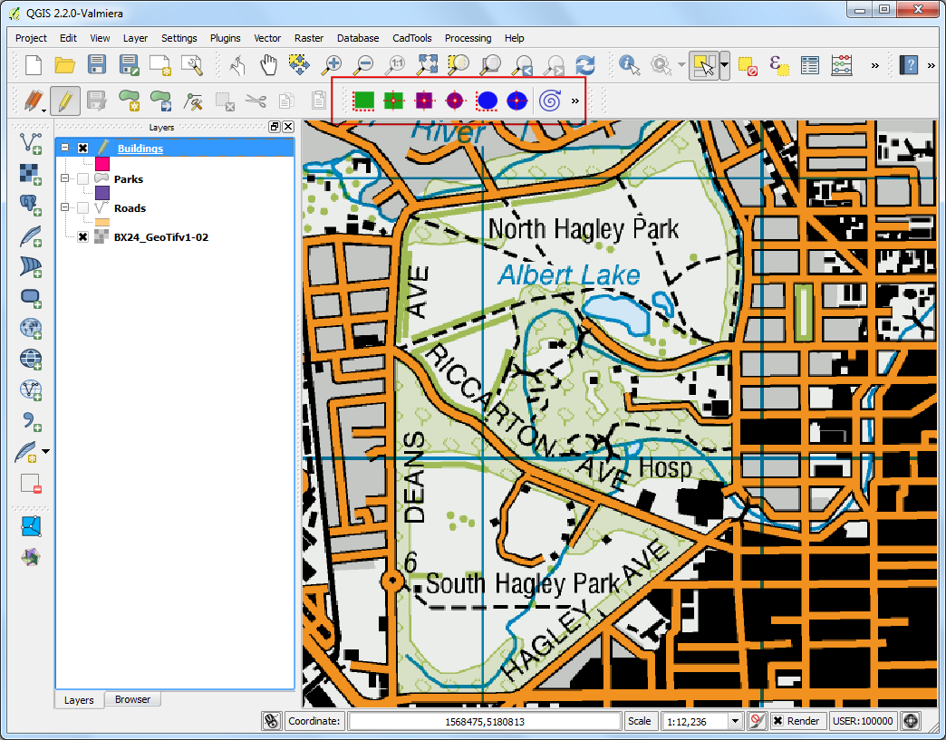
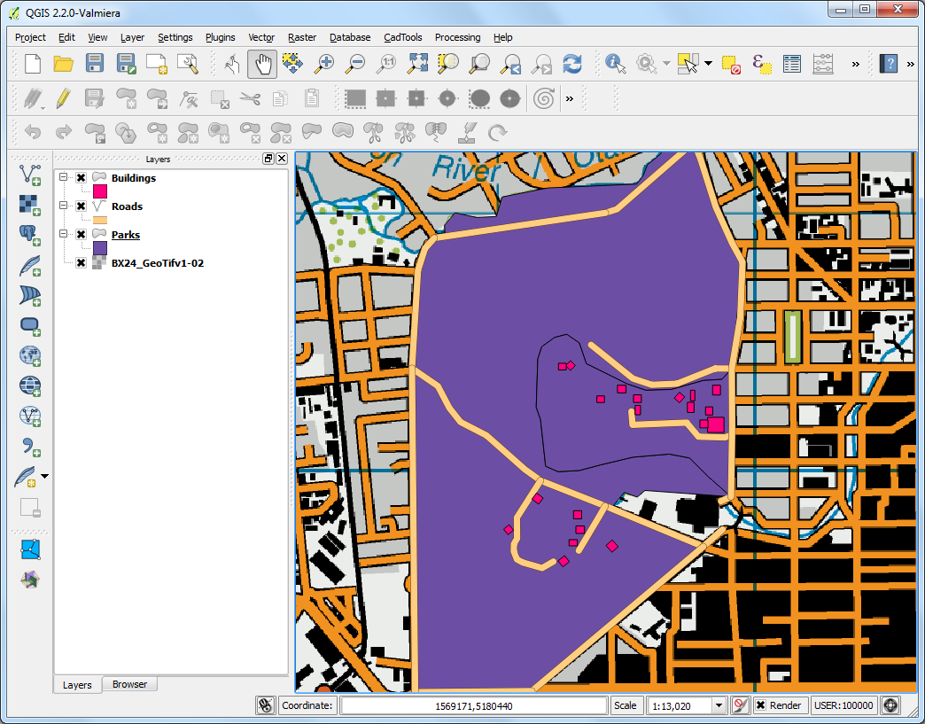
Now it is time to digitize a buildings layer. Create a new polygon layer named Buildings by going to Layer ‣ New ‣ New Spatialite Layer.

Once the Buildings layer is added, turn off the Parks and Roads layer so the base topo map is visible. Select the Buildings layer and click Toggle Editing.

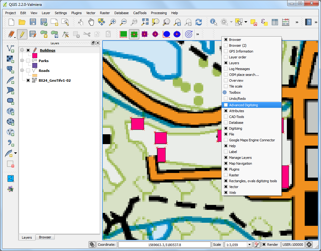
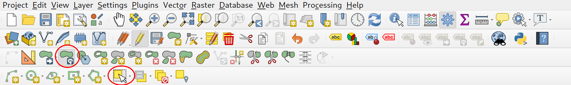
Digitizing buildings can be a cumbersome task. Also it is difficult to add vertices manually so that the edges are perpendicular and form a rectangle. We will use "Adanced Digitizing Toolbar" and "Shape Digitizing Toolbar" to help with this task. Right-click on the area with all the tools buttons above the canvas and in the menu that appears enable both toolbars (select "toolbars", not "panels" with similar names). You will see a new toolbar appear above the canvas.

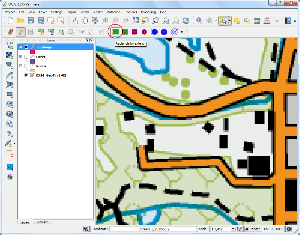
Zoom to an area with the buildings and click Rectangle by Extent button. Click and drag the mouse to draw a perfect rectangle. Similarly, add remaining buildings.

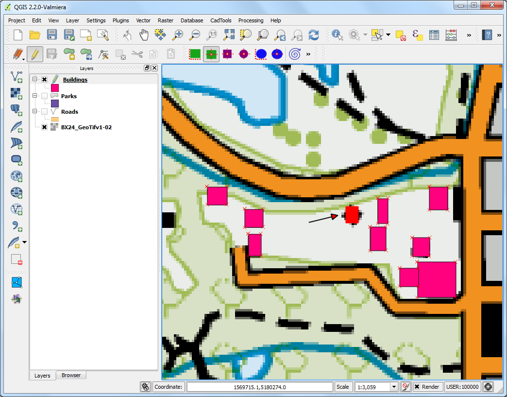
You will notice that some buildings are not vertical. We will need to draw a rectangle at an angle to match the building footprint. Click the Rectangle from center.

Click at the center of the building and drag the mouse to draw a vertical rectangle.

We need to rotate this rectangle to match the image on the topo map. The rotate tool is available in the Advanced Digitizing toolbar. Right-click on an empty area on the toolbar section and enable the Advanced Digitizing toolbar if you have not done it before.

Click the Rotate Feature(s) button.

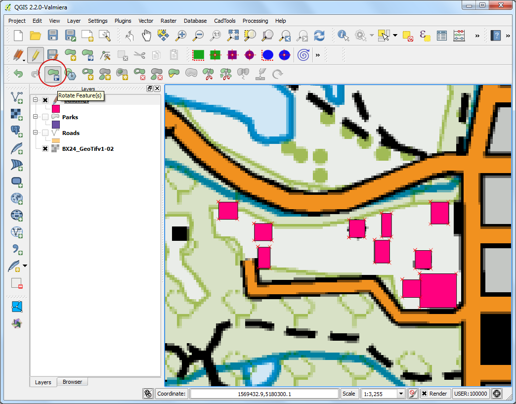
Use the Select Features by Area or Single Click tool to select the polygon that you want to rotate. Once the Rotate Feature(s) tool is activated, you will see crosshairs at the center of the polygon. Click exactly on that crosshair once, drag the mouse, and left-click again when the polygon aligns with the building footprint.

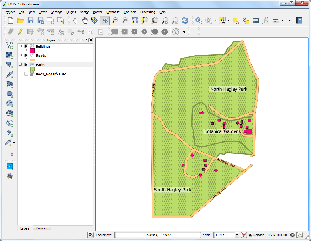
Save the layer edits and click Toggle Editing once you finish digitizing all buildings. You can drag the layers to change their order of appearance.

The digitizing task is now complete. You can play with the styling and labelling options in layer properties to create a nice looking map from the data you created.

Tutorial 2: Georeferencing Topo Sheets and Scanned Maps¶

Most GIS projects require georeferencing some raster data. Georeferencing is the process of assigning real-world coordinates to each pixel of the raster. Many times these coordinates are obtained by doing field surveys - collecting coordinates with a GPS device for few easily identifiable features in the image or map. In some cases, where you are looking to digitize scanned maps, you can obtain the coordinates from the markings on the map image itself. Using these sample coordinates or GCPs ( Ground Control Points ), the image is warped and made to fit within the chosen coordinate system. In this tutorial I will discuss the concepts, strategies and tools within QGIS to achieve a high accuracy georeferencing.

This tutorial is to geo-reference an image which has coordinates information available on the map image itself (i.e. grids with labels). If your source image does not have such information, you can use the method outlined in the next tutorial

Overview of the task¶

We will use a scanned map of southern India from 1870 and geo-reference it using QGIS.

Other skills you will learn¶

How to determine datum and coordinate system for old maps.

Get the data¶

Hipkiss’s Scanned Old Maps website has an excellent collection out-of-copyright scanned maps that one can use for research.

Download the 1870 map of southern India and save it as a JPG image on your hard drive.

For convenience, you may directly download a copy of the dataset from the link below:

1870_southern_india.jpg

Procedure¶

1. Georeferencing in QGIS is done via the Georeferencer GDAL plugin. Modern versions of QGIS have all the features of this plugin included by default, so you can skip this instruction and go to the step 2. However, if the menu option mentioned in the next step is missing, then you can follow this instruction. Georeferencer GDAL is a core plugin - meaning it is already part of your QGIS installation. You just need to enable it. Go to Plugins ‣ Manage and Install Plugins and enable the Georeferencer GDAL plugin in the Installed tab. See Using Plugins for more details on how to work with plugins.

The plugin is installed in the Raster menu. Click on Raster ‣ Georeferencer to open the plugin.

The plugin window is divided into 2 sections. The top section where the image will be displayed and the bottom section where a table showing your GCPs will appear.

Now we will open our JPG image. Go to File ‣ Open Raster. Browse to the downloaded image of the scanned map and click Open.

In the next screen, you will asked to choose the raster’s coordinate reference system (CRS). Our source image is a plain JPEG file and doesn’t have any coordinate reference system atached to it, so you can click Cancel.

You will see the image will be loaded on the top section. You can use the zoom/pan controls in the toolbar to learn more about the map.

Now we need to assign coordinates to some points on this map. If you look closely, you will see coordinate grid with markings. These are Latitude and Longitude grid lines.

Before we start adding Ground Control Points (GCP), we need to define the Transformation Settings. Go to Settings ‣ Transformation settings.

In the Transformation settings dialog, choose the Transformation type as Polynomial 2. See QGIS Documentation to learn about different transofrmation types and their uses. Click Select CRS button next to Target SRS.

If you are geo-referencing a scanned map like this, you can obtain the CRS information from the map itself. Looking at our map image, the coordinates are in Latitude/Longitude. There is no datum information given, so we have to assume an appropriate one. Since it is India and the map is quite old, we can bet the Everest 1830 datum would give us good results. Search for everest and select the CRS with oldest definition of the Everest datum (EPSG:4042). Click OK.

Note

Survey of India Topo Sheets created between the year 1960 and 2000 use the Everest 1956 spheroid and India_nepal datum. If you are georeferencing SOI Topo Sheets, , you can define a Custom CRS in QGIS with the following paramters and use it in this step. This definition includes a delta_x, delta_y and delta_z parameters for transforming this datum to WGS84. See this page for more information on the Indian Grid System.

+proj=longlat +a=6377301.243 +b=6356100.2284 +towgs84=295,736,257,0,0,0,0 +no_defs
              

Note

Most maps are created using a Projected CRS. If the map you are trying to georeference uses a projected CRS that you know of, but the graticules labels are in a Geographic CRS (latitude/longitude), you may use an alternate workflow to minimize distortion. Instead of using a Geographic CRS like we are using here, you can create a vector grid in QGIS and transform it to the projected CRS to be used as a reference for accurate coordinate capture. See this page for more details.

Name your output raster as 1870_southern_india_modified.tif. Choose LZW as the Compression. Make sure the Load in QGIS when done option is checked. CLick OK.

Note

Uncompressed GeoTIFF files can be very large in size. So compressing them is always a good idea. You can learn more about different TIFF compression options (LZW, PACKBITS or DEFLATE) in this article.

Now we can start adding the Ground Control Points (GCP). The intersections of the grid lines will serve as the ground-truth in our case. As the grid lines are labeled, we can determine the X and Y coordinates of the points using them. Click Add Point.

13 . In the pop-up window, enter the coordinates. Remember that X=longitude and Y=latitude. Click OK.

You will notice the GCP table now has a row with details of your first GCP.

Similarly, add at least more GCPs covering the entire image. The more points you have, the more accurate your image is registered to the target coordinates. The Polynomial 2 transform requires at least 6 GCPs.

Once you have added the minimum number of points required for the transform, you will notice that the GCPs now have a non-zero dX, dY and Residual error values. If a particular GCP has unusually high error values, that usually means a human-error in entering the coordinate values. So you can delete that GCP and capture it again. You can also edit the coordinate values in the GCP Table by clicking the cell in either Dest. X or Dest. Y columns. Once you are satisfied with the GCPs, go to File ‣ Start georeferencing. This will start the process of warping the image using the GCPs and creating the target raster.

Once the process finishes, you will see the georeferenced layer loaded in QGIS. The georeferencing is now complete.

Note

The GCPs will also be displayed in the main QGIS Canvas. If you wish to remove them, you can switch to the Georeferencer window, and choose File ‣ Reset Georeferencer.

It is a good practice to verify your work. How do we check if our georeferencing is accurate? In this case, you can load the boundary shapefile from a trusted source like the Natural Earth dataset and compare them. You will notice they match up pretty nicely. There is some error and it can be further improved by taking more control points, changing transformation parameters and trying a different datum.

Tutorial 3: Georeferencing Aerial Imagery¶

In the previous tutorial we covered the basic process of georeferencing in QGIS. That method involved reading the coordinates from your scanned map and entering them manually as control points. Many times though you may not have the coordinates printed on your map, or you are trying to georeference an image. In that case, you can use another georeferenced data-source as your input. In this tutorial, you will learn how to use existing open data sources in your georeferencing process.

Overview of the task¶

We will georeference high resolution balloon-imagery using reference coordinates from OpenStreetMap.

Other skills you will learn¶

Downloading super high-resolution public domain imagery.
Using XYZ Tile Layers as basemap.
Using the OSM Place Search plugin in QGIS.
Setting a custom no-data value for a layer.

Get the data¶

In this tutorial, we will be using kite and balloon imagery collected by The Public Laboratory. They make the georeferenced versions of the images also available, but we will download a non-georeferenced JPG image and go through the process of georeferencing it in QGIS.

Download the JPG image of Washington Square Park, New York. You can right-click the JPG button and choose Save link as....

For convenience, you may directly download a copy of the dataset from the link below:

newyorkcity-washingtonsquarepark.jpg

Procedure¶

We will use a basemap from OpenStreetMap to capture the coordinates for georeferencing. QGIS3 comes with built-in support for tile layers. These are commonly known as ‘XYZ’ layers since they are made using individual map tiles for each zoom level (z) on a x,y coordinate grid. You can find the OpenStreetMap layer under XYZ Tiles in the Browser Panel. Drag the layer to the main canvas. Once loaded, note the Coordinate Reference System (CRS) for this layer in the bottom-right corder. It is set as EPSG 3857 Pseudo Mercator. This is important because the coordinates we infer from this layer during georeferencing will be in this CRS.

Note

See this page for more details on XYZ layers and how to add other basemaps in QGIS.

The image we are georeferencing is for Washington Square Park, New York. You can zoom/pan try to locate this park in the map. But that is cumbersome and may not be practical. An easier way is to use the OpenStreetMap (OSM) Place Search plugin to search for the exact location. Install the OSM Place Search plugin from Plugins ‣ Manage and install plugins ‣ All. If you do not see this plugin in the search results, make sure you have checked Also show experimental plugins under Settings. See Using Plugins for more information on using plugins in QGIS.

Once the plugin is installed, you will see a new panel called OSM Place Search.... Search for Washington Square Park in the Name contains.. box and click ->. You will see the matching place names appear in the results panel. Select the correct result and click the Zoom button.

You will see the map that is familiar and contains the landmarks that we can identify from the image. You may close the OSM Place Search panel now. If you need it again, you can open it from View ‣ Panels ‣ OSM Place Search.

Now it is time to start georeferencing. Launch the Georeferencer from Raster ‣ Georeferencer ‣ Georeferencer. If you do not see that menu item, you will need to enable the Georeferencer GDAL plugin from Plugins ‣ Manage and install Plugins ‣ Installed.

In the Georeferencer window, go to File ‣ Open Raster. Navigate to the downloaded JPG file and click Open.

In the next screen, you will asked to choose the raster’s coordinate reference system (CRS). Our source image is a plain JPEG file and doesn’t have any coordinate reference system atached to it, so you can click Cancel.

Before we start adding Ground Control Points (GCP), we need to define the Transformation Settings. Go to Settings ‣ Transformation settings.

In the Transformation settings dialog, choose the Transformation type as Polynomial 2. See QGIS Documentation to learn about different transofrmation types and their uses. As noted earlier, our basemap is in EPSG 3857 Pseudo Mercator CRS, so set that as the Target CRS. You can leave the Output raster name to the default and choose LZW as the Compression. Check the Use 0 for transparency when needed. Make sure the Load in QGIS when done option is checked. CLick OK.

Now click on the Add Point button on the toolbar and select an easily identifiable location on the image. Corners, intersections, poles etc. make good control points.

Once you click on the image at a control point location, you will see a pop-up asking you to enter map coordinates. Click the button From map canvas.

Find the same location in the reference layer and click at the precise point. The coordinates are auto-populated from your click on the map canvas. Click Ok. Similarly, choose at least 6 points on the image and add their coordinates from the reference layer.

Note

Tip: When selecting a GCP on a building, always choose the bottom of the building. Many aerial and satellite imagery have leaning buildings, so choosing a point on the rooftop will introduce errors.

Once you have added the minimum number of points required for the transform, you will notice that the GCPs now have a non-zero dX, dY and Residual error values. If a particular GCP has unusually high error values, that usually means a human-error in entering the coordinate values. So you can delete that GCP and capture it again.

Once you are satisfied with the GCPs, go to File ‣ Start georeferencing. This will start the process of warping the image using the GCPs and creating the target raster.

Once the process finishes, you will see the georeferenced layer loaded in QGIS. If all went well, you will see it nicely overlay the basemap.

To make the output look nicer, let’s remove the white border. Right-click on the image layer and choose Properties.

Switch to the Transparency tab. Add 255 as the Additional no data value and click OK.

Note

8-bit images have pixel values in the range 0-255. 0 is black and 255 is white.

Now you will see your georeferenced image nicely overlaid on the base layer.

Importing Spreadsheets or CSV files (QGIS3)¶

Many times the GIS data comes in a table or an Excel spreadsheet. Also, if you have a list lat/long coordinates, you can easily import this data in your GIS project.

Overview of the task¶

We will be importing a text file of earthquake data to QGIS.

Get the data¶

NOAA’s National Geophysical Data Center produces a great dataset of all significant earthquakes since 2150 BC. Learn more.

Download Significant Earthquake Database text file.

For convenience, you may directly download a copy of both the datasets from the links below:

signif.txt

Data Source [NGDC]

Procedure¶

Examine your tabular data source. To import this data to QGIS, you will have to save it as a text file and need at least 2 columns which contain the X and Y coordinates. If you have a spreadsheet, use Save As function in your program to save it as a Tab Delimited File or a Comma Separated Values (CSV) file. Once you have the data exported this way, you can open it in a text editor such as Notepad to view the contents. In case of the Significant Earthquake Database, the data already comes as a text file which contains latitude and longitude of the earthquake centers along with other related attributes. You will see that each field is separated by a TAB.

QGIS3 comes with a unified data manager that allows you to load all the various supported data format. Click the Open Data Source Manager button on the Data Source Toolbar. You can also use Ctrl + L keyboard shortcut.

Switch to the Delimited Text tab. Click the ... button next to File name and specify the path to the text file you downloaded. In the File format section, select Custom delimiters and check Tab. The Geometry definition secction will be auto-populated if it finds a suitable X and Y coordinate fields. In our case they are LONGITUDE and LATITUDE. You may change it if the import selects the wrong fields. You can leave the Geometry CRS to the default EPSG:4326 WGS84 CRS. If your file contained coordinates in a different CRS, you can select the appropriate CRS here. Click OK.

Note

It is easy to confuse X and Y coordinates. Latitude specifies the north-south position of a point and hence it is a Y coordinate. Similarly Longitude specifies the east-west position of a point and it is a X coordinate.

You will now see that the data will be imported and displayed in the QGIS canvas as a new layer called signif.

Assignment

The purpose of the task is to get experience of the tools for editing vector data in QGIS. There are two subtasks. The first is to digitize new features from an ortophoto, the second is to create a new layer using the accidents data.

Launch QGIS and open the map from this zip-archive. Select "SWEREF99/RT90 2.5 gon V emulation" CRS for the project and for all layers (please refer to instruction in the Lab 1 assignment). You will see an ortophoto covering the areas around Campus Norrköping, a vector layer and a polygon layer showing the outlines of the study area. The task is to create three new vector layers showing water areas (polygons), trees (points) and streets (lines) in the study area.

Instructions for subtask 1
Create a new polyline layer and fill in the name street centerlines and add an attribute name. Create another layer in the same way with feature type point and the name trees and finally a third polygon layer with the name water.

Select the tree layer, zoom into the ortophoto to find the positions of the trees and enter a point in each center as accurate as possible. Digitize most of the trees that you see in the image. Continue by selecting the water layer and trace the borderlines of the different water sections as accurate as possible (zoom in). You should trace several different polygons separated by bridges and dams. You will find that it is difficult to see the shorelines in the image for your help you can use the existing line layer as support.

Tip

Maximize the QGIS window when you work and zoom in so you get high accurracy.

Use lines to draw streets. Street segments must start and stop in crossings. Use the snapping tool to connect the segments in crossings. Enter street names according to the rastermap in the table.

Instructions for subtask 2
Import the table road_accidents from the data to the view and convert the table to a point layer. A new layer should be created in the top of the table of content. Symbolize it as you see fit.

Report Make a report that describes the home assignment in the usual way. Create a map layout with a map (select an appropriate scale) together with the traditional layout elements. The map must show the three layers that you have created by digitizing and also the symbolized traffic accidents. The street names must also be added on the map but the ortophoto should not be visible.

Tutorials 1, 2, 3 and 4 are a courtesy of QGIS tutorial by Ujaval Gandhi and shared here in accordance with CC-BY 4.0 license under the same license. Thank you, Ujaval Gandhi!