Overview of Projection Support¶

QGIS has support for approximately 7,000 known CRSs. These standard CRSs are based on those defined by the European Petroleum Search Group (EPSG) and the Institut Geographique National de France (IGNF), and are made available in QGIS through the underlying “Proj” projection library. Commonly, these standard projections are identified through use of an authority:code combination, where the authority is an organisation name such as “EPSG” or “IGNF”, and the code is a unique number associated with a specific CRS. For instance, the common WGS 84 latitude/longitude CRS is known by the identifier EPSG:4326, and the web mapping standard CRS is EPSG:3857.

Custom, user-created CRSs are stored in a user CRS database. See official documentation for information on managing your custom coordinate reference systems.

Layer Coordinate Reference Systems¶

In order to correctly project data into a specific target CRS, either your data must contain information about its coordinate reference system or you will need to manually assign the correct CRS to the layer. For PostGIS layers, QGIS uses the spatial reference identifier that was specified when that PostGIS layer was created. For data supported by OGR or GDAL, QGIS relies on the presence of a recognized means of specifying the CRS. For instance, for the Shapefile format this is a file containing the Well-Known Text (WKT) representation of the layer’s CRS. This projection file has the same base name as the .shp file and a .prj extension. For example, alaska.shp would have a corresponding projection file named alaska.prj.

Whenever a layer is loaded into QGIS, QGIS attempts to automatically determine the correct CRS for that layer. In some cases this is not possible, e.g. when a layer has been provided without retaining this information. Whenever QGIS cannot automatically determine the correct CRS for a layer, it will prompt you to manually select the CRS. Selecting the correct choice is crucial, as a wrong choice will place your layer in the wrong position on the Earth’s surface! Sometimes, accompanying metadata will describe the correct CRS for a layer, in other cases you will need to contact the original author of the data to determine the correct CRS to use.

Project Coordinate Reference Systems¶

Every project in QGIS also has an associated Coordinate Reference System. The project CRS determines how data is projected from its underlying raw coordinates to the flat map rendered within your QGIS map canvas. Behind the scenes, QGIS transparently reprojects all layers contained within your project into the project’s CRS, so that they will all be rendered in the correct position with respect to each other!

It is important to make an appropriate choice of CRS for your QGIS projects. Choosing an inappropriate CRS can cause your maps to look distorted, and poorly reflect the real-world relative sizes and positions of features. Usually, while working in smaller geographic areas, there will be a number of standard CRSs used within a particular country or administrative area. It’s important to research which CRSs are appropriate or standard choices for the area you are mapping, and ensure that your QGIS project follows these standards.

The project CRS can be set through the CRS tab of the Project properties dialog (Project ‣ Properties…). It will also be shown in the lower-right of the QGIS status bar.

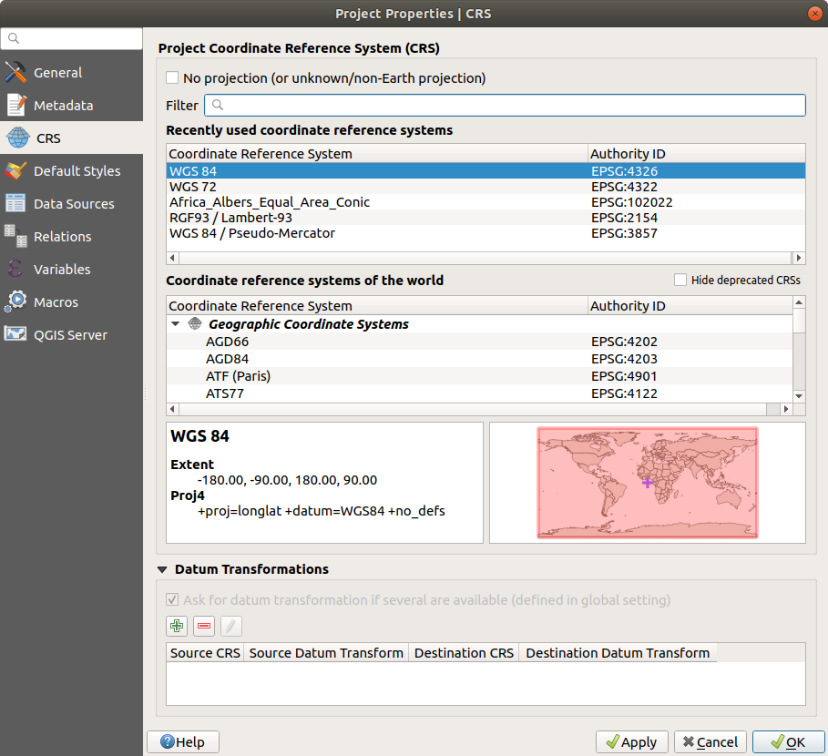
Project Properties Dialog

The CRS tab also has an optional setting for No projection. Checking this setting will disable ALL projection handling within the QGIS project, causing all layer and map coordinates to be treated as simple 2D Cartesian coordinates, with no relation to positions on the Earth’s surface.

Whenever you select a new CRS for your QGIS project, the measurement units will automatically be changed in the General tab of the Project properties dialog (Project ‣ Properties…) to match the selected CRS. For instance, some CRSs define their coordinates in feet instead of meters, so setting your QGIS project to one of these CRSs will also set your project to measure using feet by default.

CRS Settings¶

By default, QGIS starts each new project using a global default projection. This default CRS is EPSG:4326 (also known as “WGS 84”), and it is a global latitude/longitude based reference system. This default CRS can be changed via the CRS for New Projects setting in the CRS tab under Settings ‣ Options. There is an option to automatically set the project’s CRS to match the CRS of the first layer loaded into a new project, or alternatively you can select a different default CRS to use for all newly created projects. This choice will be saved for use in subsequent QGIS sessions.

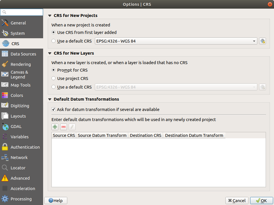
The CRS tab in the QGIS Options Dialog

When you use layers that do not have a CRS, you can define how QGIS responds to these layers. This can be done globally in the CRS tab under Settings ‣ Options.

The options shown in figure_projection_options are:

• Prompt for CRS
• Use project CRS
• Use a default CRS

If you want to define the Coordinate Reference System for a certain layer without CRS information, you can also do that in the Source tab of the raster and vector properties dialog (see Source Properties for rasters and Source Properties for vectors). If your layer already has a CRS defined, it will be displayed as shown in Source tab in vector Layer Properties dialog. Note that changing the CRS in this setting does not alter the underlying data source in any way, rather it just changes how QGIS interprets the raw coordinates from the layer in the current QGIS project only.

On The Fly (OTF) CRS Transformation¶

QGIS supports “on the fly” CRS transformation for both raster and vector data. This means that regardless of the underlying CRS of particular map layers in your project, they will always be automatically transformed into the common CRS defined for your project.

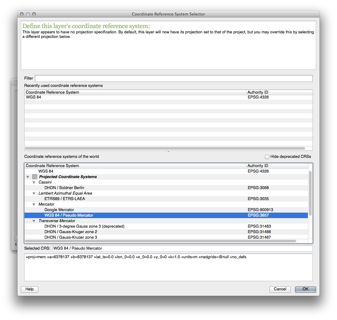
Coordinate Reference System Selector¶

This dialog helps you assign a Coordinate Reference System to a project or a layer, provided a set of projection databases. Items in the dialog are:

• Filter: If you know the EPSG code, the identifier, or the name for a Coordinate Reference System, you can use the search feature to find it. Enter the EPSG code, the identifier or the name.
• Recently used coordinate reference systems: If you have certain CRSs that you frequently use in your everyday GIS work, these will be displayed in this list. Click on one of these items to select the associated CRS.
• Coordinate reference systems of the world: This is a list of all CRSs supported by QGIS, including Geographic, Projected and Custom coordinate reference systems. To define a CRS, select it from the list by expanding the appropriate node and selecting the CRS. The active CRS is preselected.
• PROJ text: This is the CRS string used by the PROJ projection engine. This text is read-only and provided for informational purposes.

The CRS selector also shows a rough preview of the geographic area for which a selected CRS is valid for use. Many CRSs are designed only for use in small geographic areas, and you should not use these outside of the area they were designed for. The preview map shades an approximate area of use whenever a CRS is selected from the list. In addition, this preview map also shows an indicator of the current main canvas map extent.

Datum Transformations¶

In QGIS, ‘on-the-fly’ CRS transformation is enabled by default, meaning that whenever you use layers with different coordinate systems QGIS transparently reprojects them to the project CRS. For some CRS, there are a number of possible transforms available to reproject to the project’s CRS! QGIS optionally allows you to define a particular transformation to use, otherwise QGIS uses a default one.

This customization is done in the Settings ‣ Options –> CRS tab menu under the Default datum transformations group:

• using Ask for datum transformation if several are available: when more than one appropriate datum transformation exists for a source/destination CRS combination, a dialog will automatically be opened prompting users to choose which of these datum transformations to use for the project;

• or predefining a list of the appropriate default transformations to use when loading layers to projects or reprojecting a layer.

  Use the button to open the Select Datum Transformations dialog. Then:

  1. Indicate the Source CRS of the layer, using the drop-down menu or the ^{Select CRS} widget.

  2. Likewise, provide the Destination CRS.

  3. Depending on the transform grid files (based on GDAL and PROJ version installed on your system), a list of available transformations from source to destination is built in the table. Clicking a row shows details on the settings applied (epsg code, accuracy of the transform, number of stations involved…).

     You can choose to only display current valid transformations by checking the Hide deprecated option.

  4. Find your preferred transformation, select it and click OK.

     A new row is added to the table under CRS ‣ Default datum transformations with information about ‘Source CRS’ and ‘Destination CRS’ as well as ‘Source datum transform’ and ‘Destination datum transform’.

  From now, QGIS automatically uses the selected datum transformation for further transformation between these two CRSs until you remove it from the list or replace it with another one.

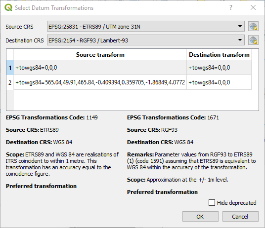
Selecting a preferred default datum transformation

Datum transformations set in the Settings ‣ Options –> CRS tab will be inherited by all new QGIS projects created on the system. Additionally, a particular project may have its own specific set of transformations specified via the CRS tab of the Project properties dialog (Project ‣ Properties…). These settings apply to the current project only.

1. Projections¶

The CRS that all the data as well as the map itself from Lab 2 Tutorial 3 is called WGS84. This is a very common Geographic Coordinate System (GCS) for representing data. But there’s a problem, as we will see.

Download the data in this zip-archive

1. Open the map of the world which you’ll find in world/world.qgs
2. Zoom in to South Africa by using the Zoom In tool
3. Try setting a scale in the Scale field, which is in the Status Bar along the bottom of the screen. While over South Africa, set this value to 1:5 000 000 (one to five million).
4. Pan around the map while keeping an eye on the Scale field

Notice the scale changing? That’s because you’re moving away from the one point that you zoomed into at 1:5 000 000, which was at the center of your screen. All around that point, the scale is different.

To understand why, think about a globe of the Earth. It has lines running along it from North to South. These longitude lines are far apart at the equator, but they meet at the poles.

In a GCS, you’re working on this sphere, but your screen is flat. When you try to represent the sphere on a flat surface, distortion occurs, similar to what would happen if you cut open a tennis ball and tried to flatten it out. What this means on a map is that the longitude lines stay equally far apart from each other, even at the poles (where they are supposed to meet). This means that, as you travel away from the equator on your map, the scale of the objects that you see gets larger and larger. What this means for us, practically, is that there is no constant scale on our map!

To solve this, let’s use a Projected Coordinate System (PCS) instead. A PCS “projects” or converts the data in a way that makes allowance for the scale change and corrects it. Therefore, to keep the scale constant, we should reproject our data to use a PCS.

2. “On the Fly” Reprojection¶

By default, QGIS reprojects data “on the fly”. What this means is that even if the data itself is in another CRS, QGIS can project it as if it were in a CRS of your choice.

You can change the CRS of the project by clicking on button in the bottom right corner of QGIS.

1. In the dialog that appears, type the word global into the Filter field. One CRS (NSIDC EASE-Grid 2.0 Global, EPSG:6933) should appear in the list below.

2. Click on the NSIDC EASE-Grid 2.0 Global to select it, then click OK.

   Notice how the shape of South Africa changes. All projections work by changing the apparent shapes of objects on Earth.

3. Zoom in to a scale of 1:5 000 000 again, as before.

4. Pan around the map.

   Notice how the scale stays the same!

“On the fly” reprojection is also used for combining datasets that are in different CRSs.

1. Add another vector layer to your map which has the data for South Africa only. You’ll find it as world/RSA.shp.
2. Load it and a quick way to see what is its CRS is by hovering the mouse over the layer in the legend. It is EPSG:3410.

What do you notice?

The layer is visible even if it has a different CRS from the continents one.

3. Saving a Dataset to Another CRS¶

Sometimes you need to export an existing dataset in another CRS. As we will see in the next lesson, if you need to make some distance calculations on layer, it is always better to have the layer in a projected coordinate system.

Be aware that the ‘on the fly’ reprojection is related to the project and not to single layers. This means that layers can have different CRS from the project even if you see them in the correct position.

But you can easily export the layer in another CRS.

1. Open the map from Lab 2 Tutorial 3.

2. Right-click on the buildings layer in the Layers panel

3. Select Export ‣ Save Features As… in the menu that appears. You will be shown the Save Vector Layer as… dialog.

4. Click on the Browse button next to the File name field

5. Specify the name of the new layer as buildings_reprojected.shp.

6. We must change the value of the CRS. Only the recent CRSs used will be shown in the drop down menu. Click on the button next to the dropdown menu.

7. The CRS Selector dialog will now appear. In its Filter field, search for 34S.

8. Select WGS 84 / UTM zone 34S from the list

   

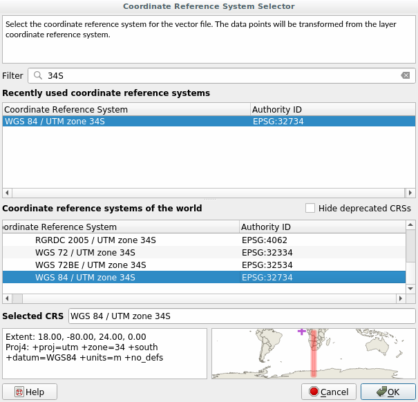
9. Leave the other options unchanged. The Save Vector Layer as… dialog now looks like this:

   

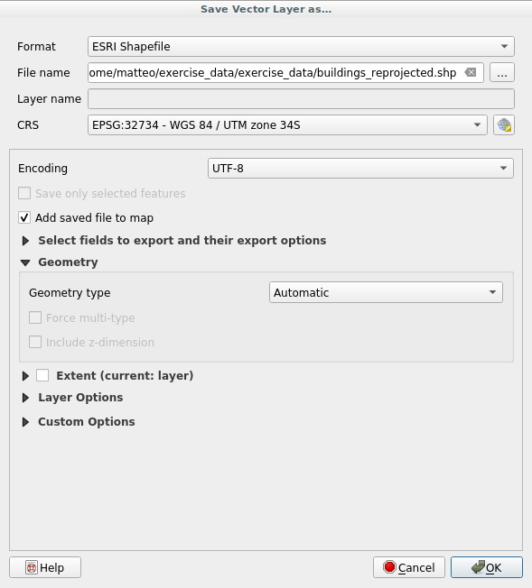
10. Click OK

You can now compare the old and new projections of the layer and see that they are in two different CRS but they are still overlapping.

4. Creating Your Own Projection¶

There are many more projections than just those included in QGIS by default. You can also create your own projections.

1. Start a new map

2. Load the world/oceans.shp dataset

3. Go to Settings ‣ Custom Projections… and you’ll see this dialog.

   

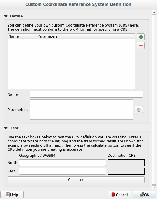
4. Click on the button to create a new projection

5. An interesting projection to use is called Van der Grinten I. Enter its name in the Name field.

   This projection represents the Earth on a circular field instead of a rectangular one, as most other projections do.

6. Add the following string in the Parameters field:

   +proj=vandg +lon_0=0 +x_0=0 +y_0=0 +R_A +a=6371000 +b=6371000 +units=m +no_defs
                 

   

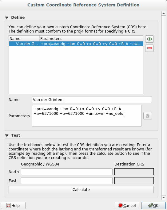
7. Click OK

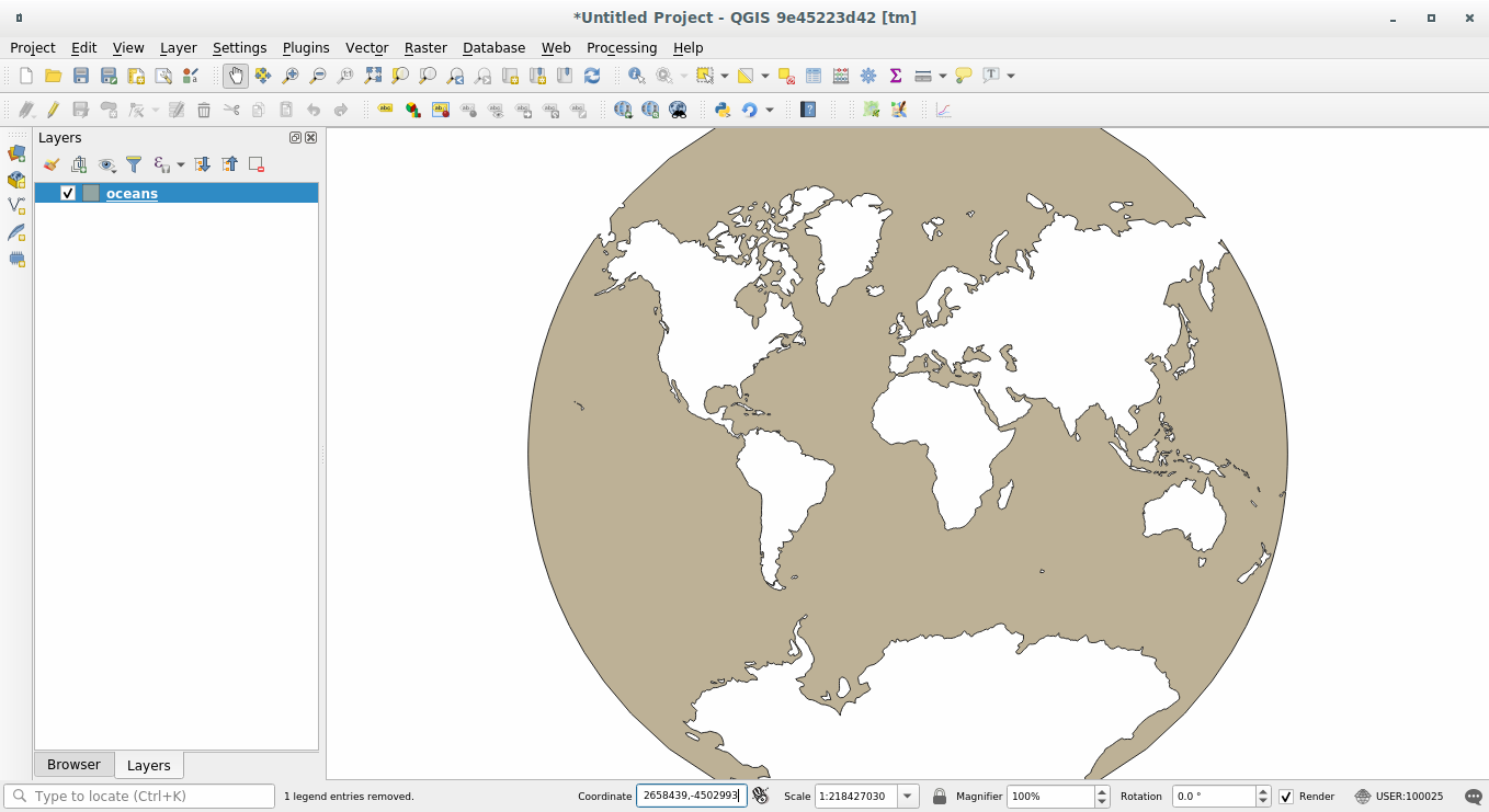
8. Click on the button to change the project CRS

9. Choose your newly defined projection (search for its name in the Filter field)

10. On applying this projection, the map will be reprojected thus:

    

5. In Conclusion¶

Different projections are useful for different purposes. By choosing the correct projection, you can ensure that the features on your map are being represented accurately.

6. Further Reading¶

Some materials for this lesson were taken from this article.

Further information on Coordinate Reference Systems is available here.

Overview of the task¶

The task is to re-project and overlay data layers of difference projections together in QGIS.

Get the data¶

Natural Earth has Admin 0 - Countries dataset. Download the countries

UK’s Ordnance Survey provides open data for download. Download the MiniScale raster product for Great Britain and extract it to a folder on your computer.

For convenience, you may directly download a copy of the dataset from the link below:

ne_10m_admin_0_countries.zip

minisc_gb.zip (Contains only the files required for this tutorial)

Data Sources: [NATURALEARTH] [OSOPENDATA]

Procedure¶

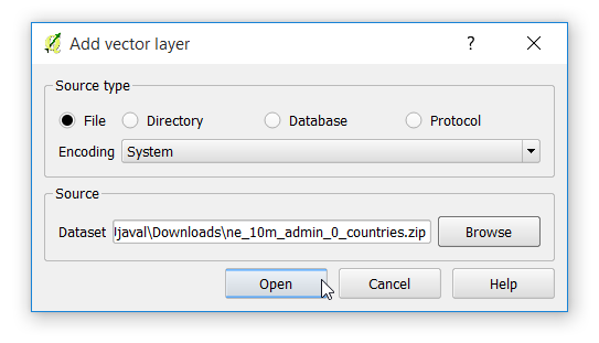
1. Open QGIS. Go to Layer ‣ Add Layer ‣ Add Vector Layer....

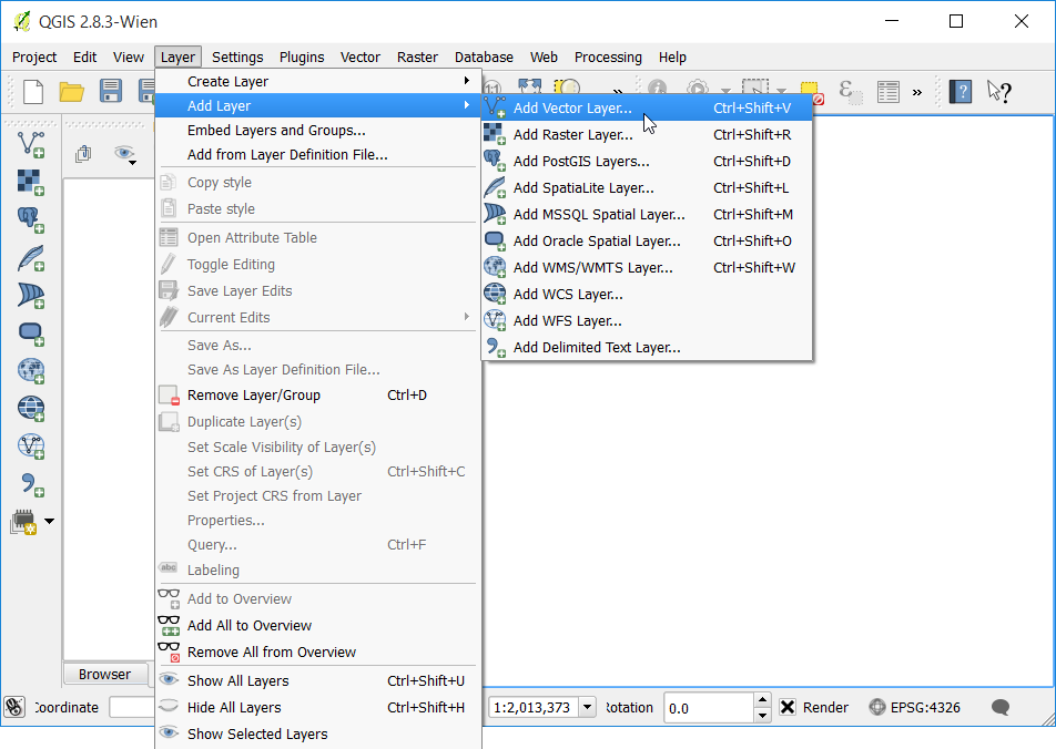
2. Browse to the downloaded ne_10m_admin_0_countries.zip file and click Open.

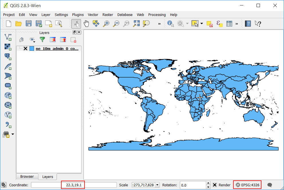
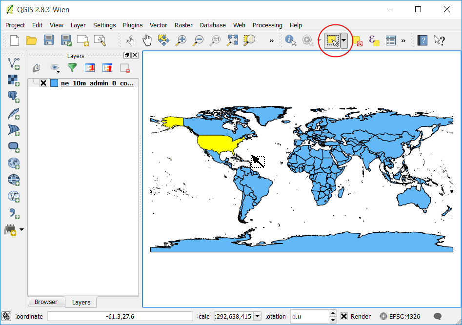
3. At the bottom of QGIS window, you will notice the label Coordinate. As you move your cursor over the map, it will show you the X and Y coordinates at that location. At the bottom-right corner you will see EPSG:4326. This is the code for the current CRS (Projection) for the project.

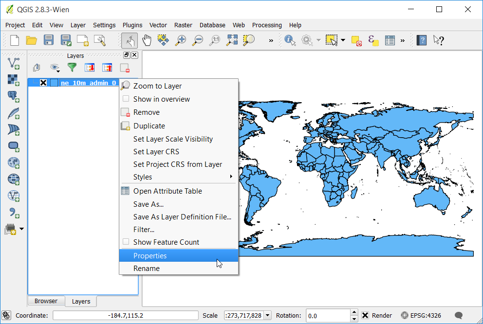
4. As you will later see, the project’s CRS may not match the layer’s CRS. To determine a layer’s projection, we can look into the metadata. Right click on ne_10m_admin_0_countries layer and select Properties.

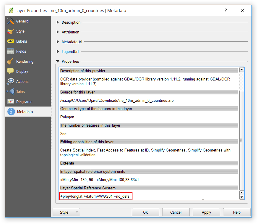
5. Switch to the Metadata tab in the Layer Properties dialog. Expand the Properties section. At the bottom, you will see the definition for the projection under Layer Spatial Reference System. This definition is in the PROJ.4 format.

6. Now let’s see how we can change the layer’s projection. This operation is called Re-Projection. Rather than re-projecting the entire layer, we can also re-project some features from the layer. Use the Select features by area or single click tool and click on United States feature to select it.

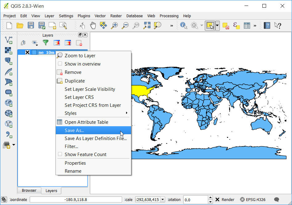
7. Right-click the ne_10m_admin_0_countries layer and select Save As.

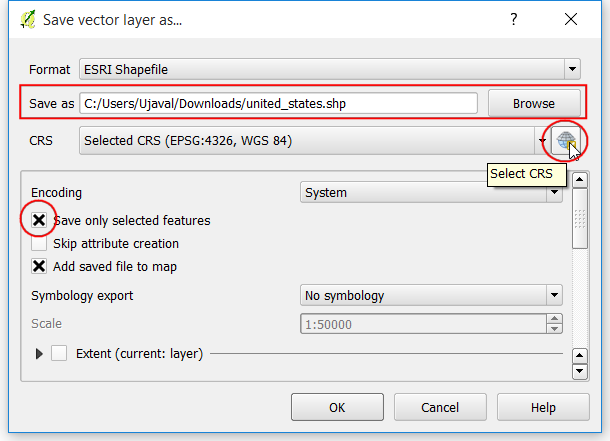
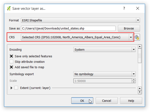
8. In the Save vector layer as... dialog, name the output layer as united_states.shp. Also check the Save only selected features box. This will ensure that only the selected feature gets re-projected and exported. Next, we choose the new projection for the layer. Click on the Select CRS button.

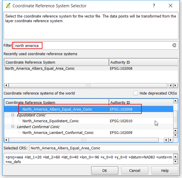
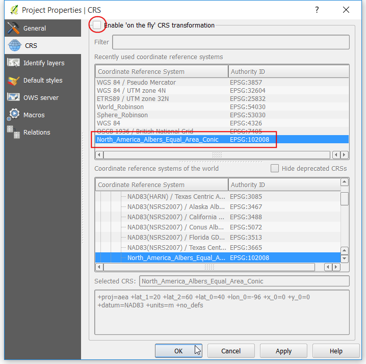
9. In the Coordinate Reference System Selector dialog, enter north america in the Filter search box. Scroll through the results and select North_America_Albers_Equal_Area_Conic (EPSG:102008) projection and click OK.

10. You will see the new CRS selected in the Save vector layer as... dialog. Click OK.

11. Once the re-projected layer gets loaded, you will notice that the new united_states layer overlays perfectly on top of ne_10m_admin_0_countries layer - even though they are in different projections. This is because QGIS has a feature called On-the-fly CRS transformation. The projection text at the bottom-right of QGIS now has the words OTF next the EPSG:4326`. To learn more, let’s explore the CRS option in QGIS.

12. Go to Settings ‣ Options....

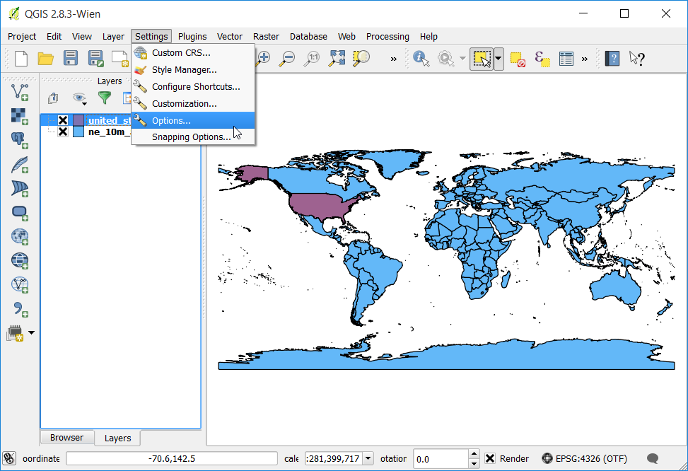
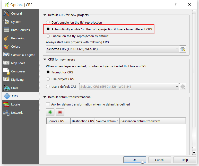
13. Switch to the CRS tab in the Options dialog. You will see that the default is Automatically enable ‘on the fly’ reprojection if the layers have different CRS. This means that when QGIS detects that you have loaded layers with different CRS, it will automatically re-project them back to a common CRS so they line up with each other. Click OK.

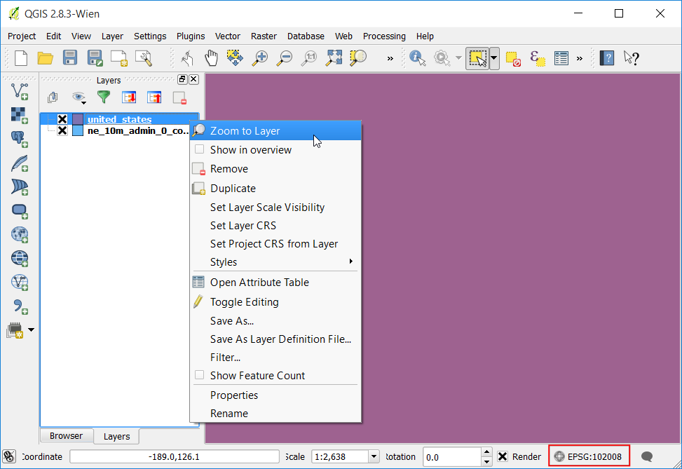
14. Let’s turn-off the On-the-fly CRS transformation and see what happens. Click on the Current CRS text at the bottom-right corner.

15. In the Project Properties dialog, un-check the Enable ‘on the fly’ CRS transformation box and click OK.

16. Back in the main QGIS window, you will see the nice world map disappear. This is because the Project CRS changed to North_America_Albers_Equal_Area_Conic and the coordinates and scale are different now. Right-click the united_states layer and select Zoom to Layer.

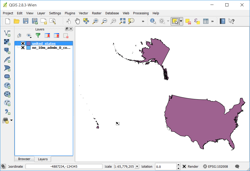
17. Now you will see the United States in the selected projection. Notice that the features from ne_10m_admin_0_countries do not appear on the canvas as they are in a different coordinate space than the united_states layer. Go back to the Project Properties dialog and turn-on the Enable ‘on the fly’ CRS transformation option for the remainder of the tutorial.

18. Now let’s switch gears and add a raster layer to our project. Browse to the directory where you had extracted the minisc_gb.zip file. Locate the RGB_TIF_COMPRESSED folder containing tif files. You will notice that the .tif image files are plain TIF files, not GeoTIFF files. That means they do not have any projection information. To use these images in a GIS, you need to georeference them. A georeference contains 2 types of information - image extents and projection. Typically, the extents are stored in a file known as World file and they have extensions like .tfw or .jgw. Most GIS software, including QGIS would be able to use information stored in the world files as long as they are stored in the same directory as the original image and has the same name. The .tfw files for the MiniScale raster files are in a separate folder named georeferencing_files.

19. Go to the ESRI_TFW_FILES folder within georeferencing_files. The .tfw files are plain text files. Open one of the .tfw files in a text editor.

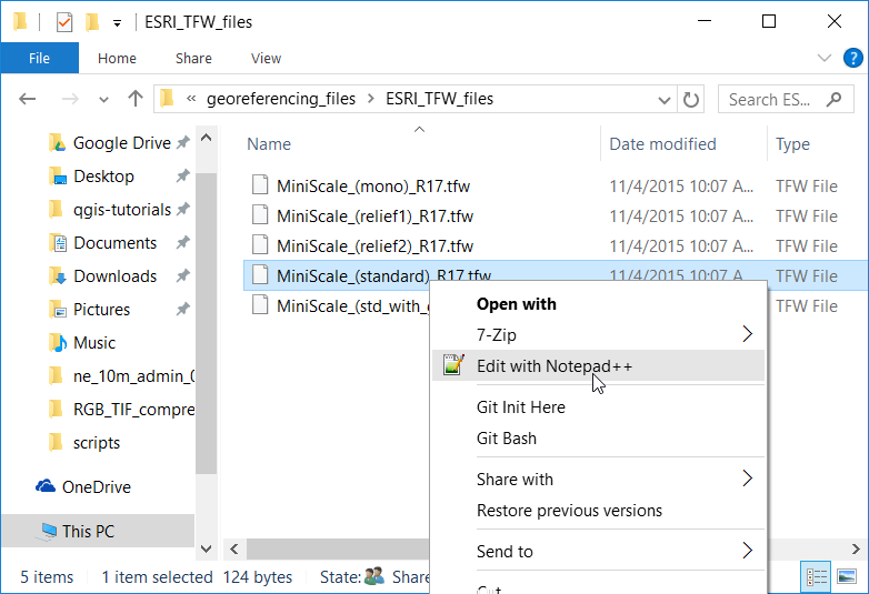
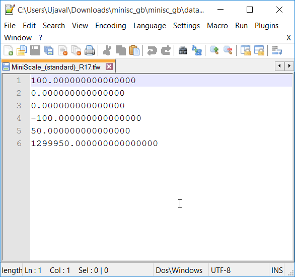
20. The world files contain 6 lines with some numbers. As explained below, each line signifies some information about the raster file. Knowing this format is useful because some data do not come with the world files and you may have to create these by hand using the supplied information.

Line 1: A: pixel size in the x-direction in map units/pixel
              Line 2: D: rotation about y-axis
              Line 3: B: rotation about x-axis
              Line 4: E: pixel size in the y-direction in map units
              Line 5: C: x-coordinate of the center of the upper left pixel
              Line 6: F: y-coordinate of the center of the upper left pixel
              

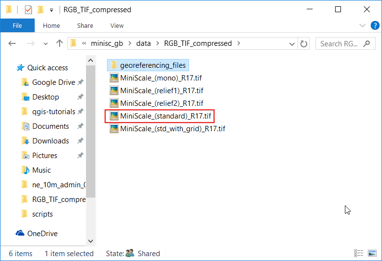
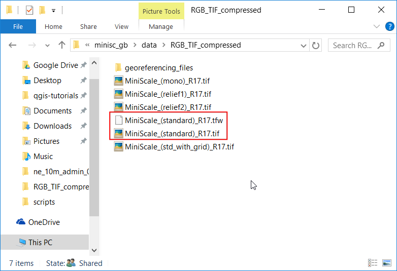
21. Copy the MiniScale_(standard)_R17.tfw file from the georeferencing_files folder to the RGB_TIF_COMPRESSED folder. This way the .tfw and the .tif files are in the same directory and QGIS can use the information.

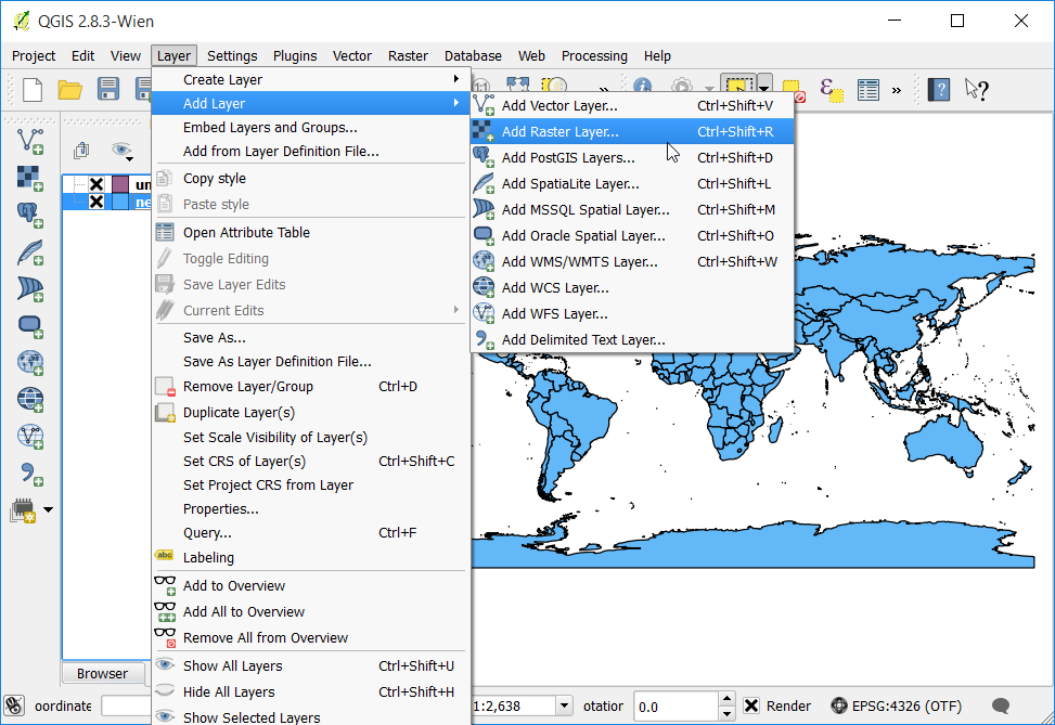
22. In the QGIS main windows, go to Layer ‣ Add Layer ‣ Add Raster Layer.... Browse to the MiniScale_(standard)_R17.tif file and click Open.

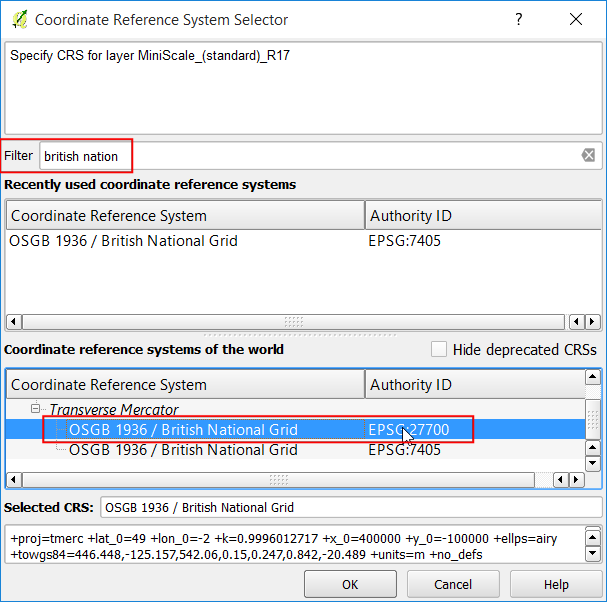
23. The Ordnance Survey files are in the British National Grid projection. In the Coordinate Reference System Selector dialog, search for british national and pick the OSGB 1936 / British National Grid (EPSG:27700) CRS. Click OK.

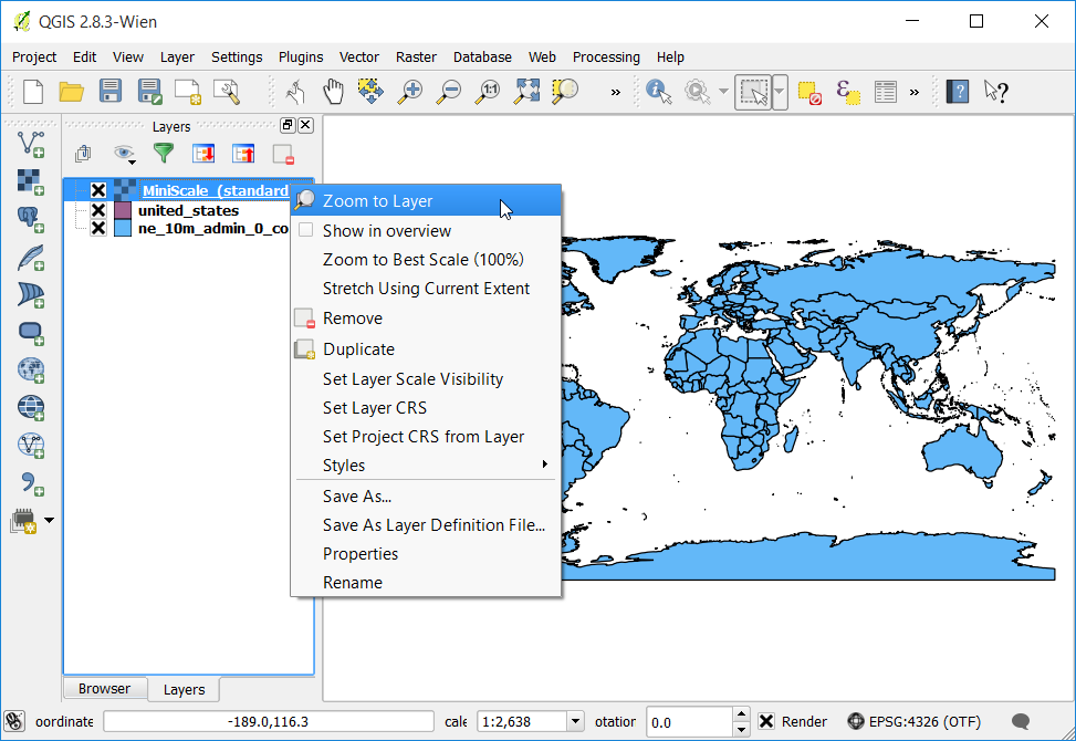
24. Once the MiniScale_(standard)_R17 layer is loaded, right-click on it and select Zoom to layer.

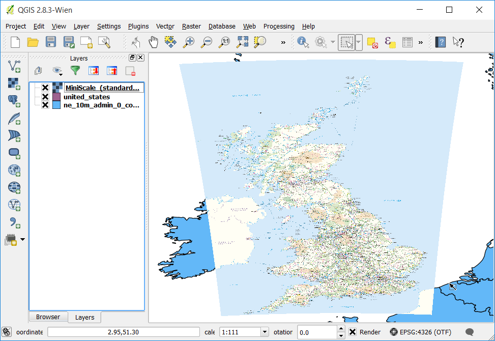
25. You will see the raster layer overlaid on top of the ne_10m_admin_0_countries vector layer. Since we have the OTF enabled with EPSG:4326, the MiniScale_(standard)_R17 layer gets dynamically reprojected to EPSG:4326 and shown in the same coordinate space as the other layer.

1. Follow Along: Loading a WMS Layer¶

For this exercise, you can either use the result of Lab 2 Tutorial 3 or use again this base map, or just start a new map and load some existing layers into it. For this example, we used a new map and loaded the original places and landuse layers and adjusted the symbology:

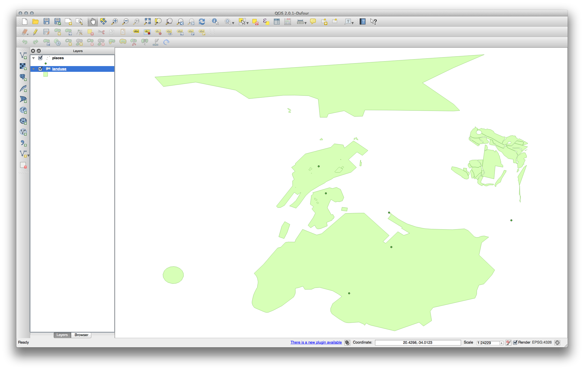
• Load these layers into a new map, or use your original map with only these layers visible.

• Before starting to add the WMS layer, first deactivate “on the fly” projection. This may cause the layers to no longer overlap properly, but don’t worry: we’ll fix that later.

• To add WMS layers, click on the Add WMS Layer button:

  

• To create a new connection to a WMS, click on the New button.

You’ll need a WMS address to continue. There are several free WMS servers available on the Internet. One of these is terrestris, which makes use of the OpenStreetMap dataset.

• To make use of this WMS, set it up in your current dialog, like this:

  

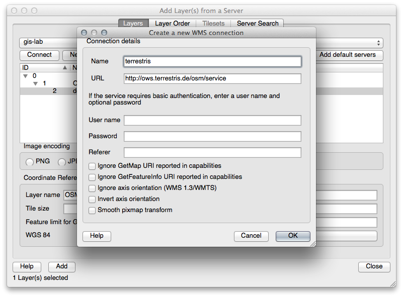
• The value of the Name field should be terrestris.

• The value of the URL field should be http://ows.terrestris.de/osm/service.

• Click OK. You should see the new WMS server listed:

  

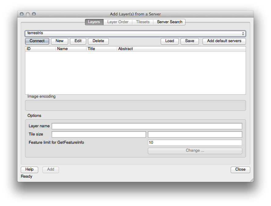
• Click Connect. In the list below, you should now see these new entries loaded:

  

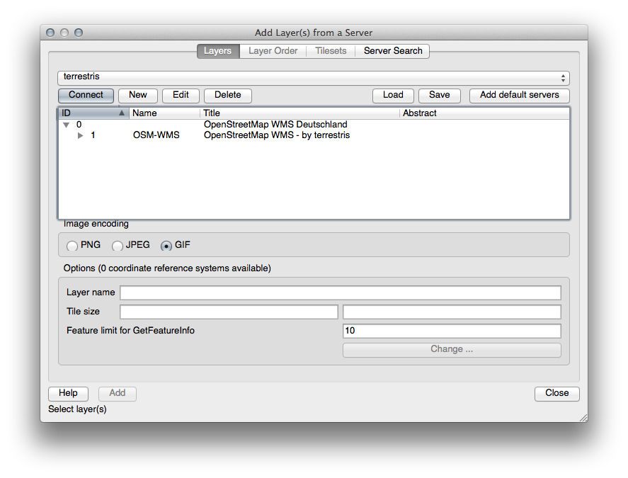
  These are all the layers hosted by this WMS server.

• Click once on the OSM-WMS layer. This will display its Coordinate Reference System:

  

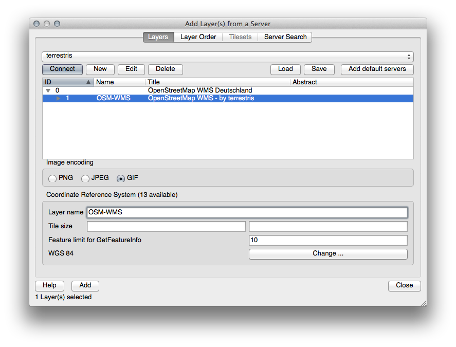
Since we’re not using WGS 84 for our map, let’s see all the CRSs we have to choose from.

• Click the Change button. You will see a standard Coordinate Reference System Selector dialog.

• We want a projected CRS, so let’s choose WGS 84 / Pseudo Mercator.

  

• Click OK.

• Click Add and the new layer will appear in your map as OSM-WMS.

• In the Layers list, click and drag it to the bottom of the list.

You will notice that your layers aren’t located correctly. This is because “on the fly” projection is disabled. Let’s enable it again, but using the same projection as the OSM-WMS layer, which is WGS 84 / Pseudo Mercator.

• Enable “on the fly” projection.

• In the CRS tab (Project Properties dialog), enter the value pseudo in the Filter field: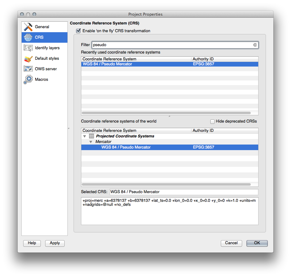

  

• Choose WGS 84 / Pseudo Mercator from the list.

• Click OK.

• Now right-click on one of your own layers in the Layers list and click Zoom to layer extent. You should see the Swellendam area:

  

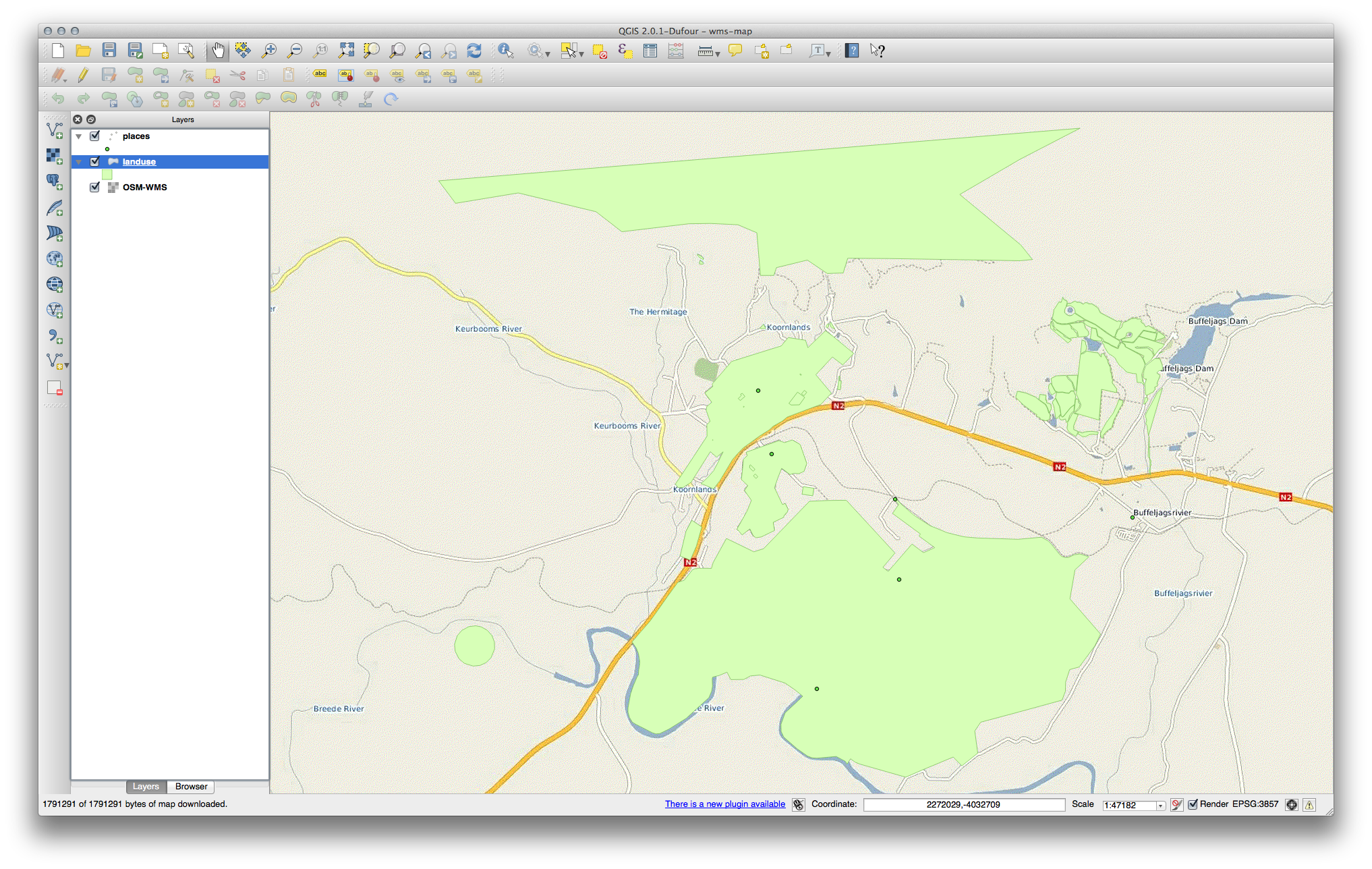
Note how the WMS layer’s streets and our own streets overlap. That’s a good sign!

2. Try Yourself¶

• Hide the OSM-WSM layer in the Layers list.

• Add the “ZAF CGS 1M Bedrock Lithostratigraphy” WMS server at this URL: http://196.33.85.22/cgi-bin/ZAF_CGS_Bedrock_Geology/wms

• Load the BEDROCKGEOLOGY layer into the map (use the Add WMS Layer button as before). Remember to check that it’s in the same WGS 84 / World Mercator projection as the rest of your map!

• You might want to set its Encoding to JPEG and its Tile size option to 200 by 200, so that it loads faster: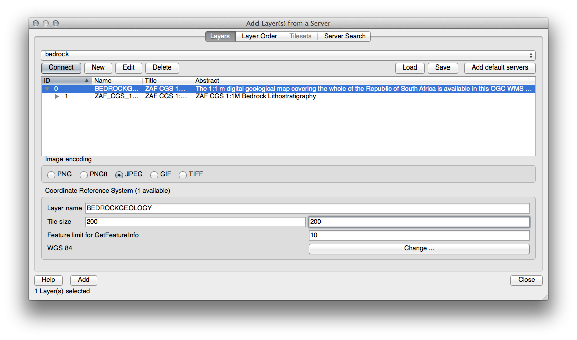

  

3. Try Yourself¶

• Hide all other WMS layers to prevent them rendering unnecessarily in the background.
• Add the “OGC” WMS server at this URL: http://ogc.gbif.org:80/wms
• Add the bluemarble layer.